IF is a Google Sheets function that acts based on a given condition. You provide a boolean and tell what to do based on whether it’s TRUE or FALSE. You can combine IF with other logical functions – AND, OR – to create nested formulas and go over multiple sets of criteria. But should you? IFS is a dedicated function, which evaluates multiple conditions to return a value. However, sometimes nested IF statements do better than IFS. Let’s explore some real-life examples and find out which logical function is a go.
If you prefer watching to reading, check out this simple tutorial by Railsware Product Academy on how to use the IF function (IFS, Nested IFs) in Google Sheets.
IF Google Sheets function explained
IF Google Sheets syntax
=IF(logical_expression, value_if_true, value_if_false)
IF function in Google Sheets evaluates one logical expression and returns a value depending on whether the expression is true or false. value_if_false is blank by default.
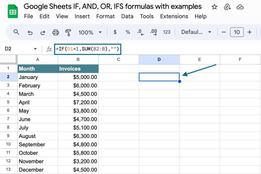
Google Sheets IF formula example
=IF(D1=1,SUM(B2:B),"")
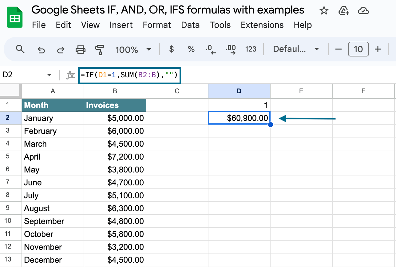
Interpretation of the Google Sheets IF formula:
If the value in the D1 cell equals one (logical_expression), then the formula will count the sum of values in the range B2:B (value_if_true). Otherwise, the formula will return an empty cell (value_if_false).
Google Sheets IF THEN formula
There is no specific Google Sheets IF THEN formula. Sometimes IF and IF THEN are used interchangeably. In many programming languages, IF THEN is used as a common phrase to say ‘If this happens, do that.’
In Google Sheets, the IF function naturally does what an IF THEN function suggests.
=IF(logical_expression, value_if_true, value_if_false)
When you use an IF function, the action taken for a true condition is essentially the ‘THEN’ part. For example, in IF(A1 > 10, "Yes", "No"), the “Yes” is what happens ‘THEN’ if A1 is greater than 10.
Nested IF Google Sheets statements for multiple logical expressions
Let’s say you need to evaluate multiple logical expressions. For this, you can nest multiple IF statements Google Sheets in a single formula. It may look as follows:
=IF(logical_expression#1, value_if_true,
IF(logical_expression#2, value_if_true,
IF(logical_expression#3, value_if_true,
IF(logical_expression#4,value_if_true,value_if_false))))
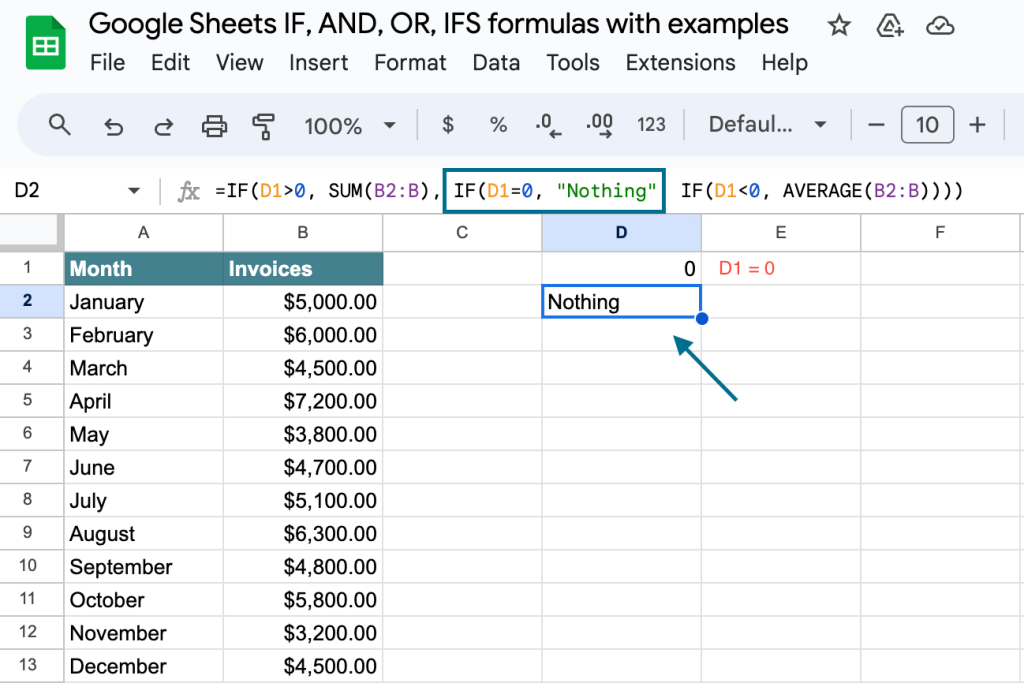
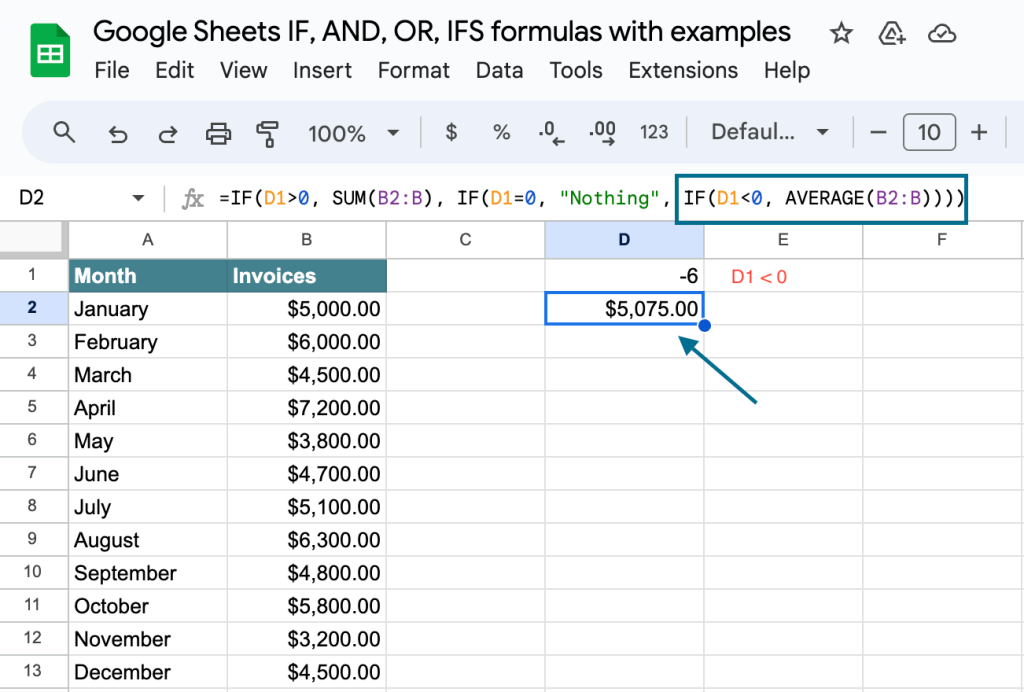
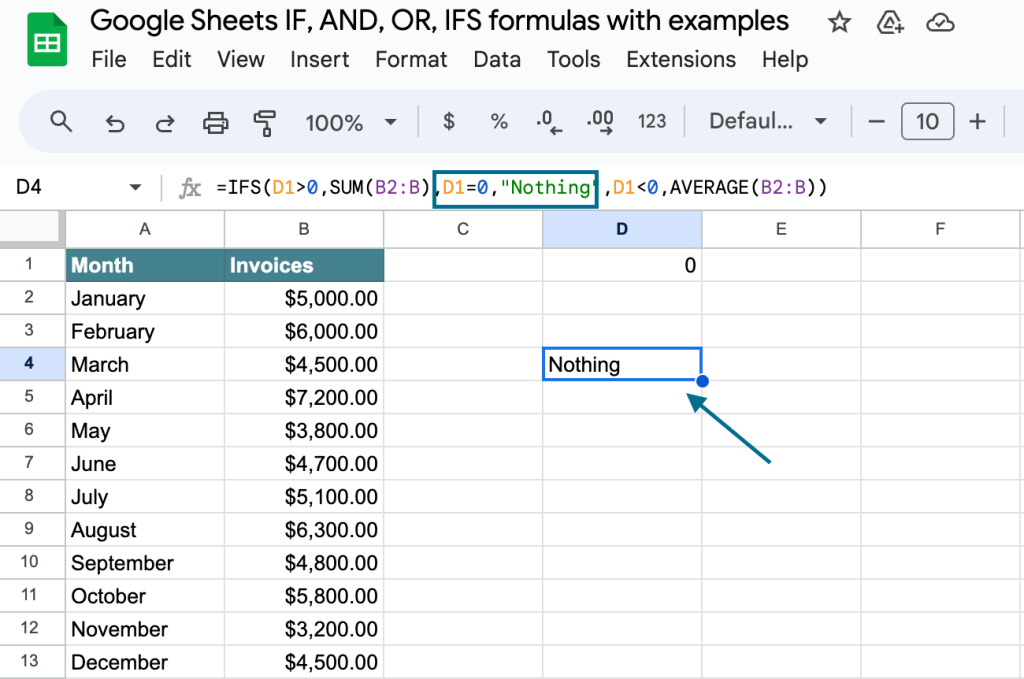
Example of a nested IF formula Google Sheets
=IF(D1>0, SUM(B2:B), IF(D1=0, "Nothing", IF(D1<0, AVERAGE(B2:B))))
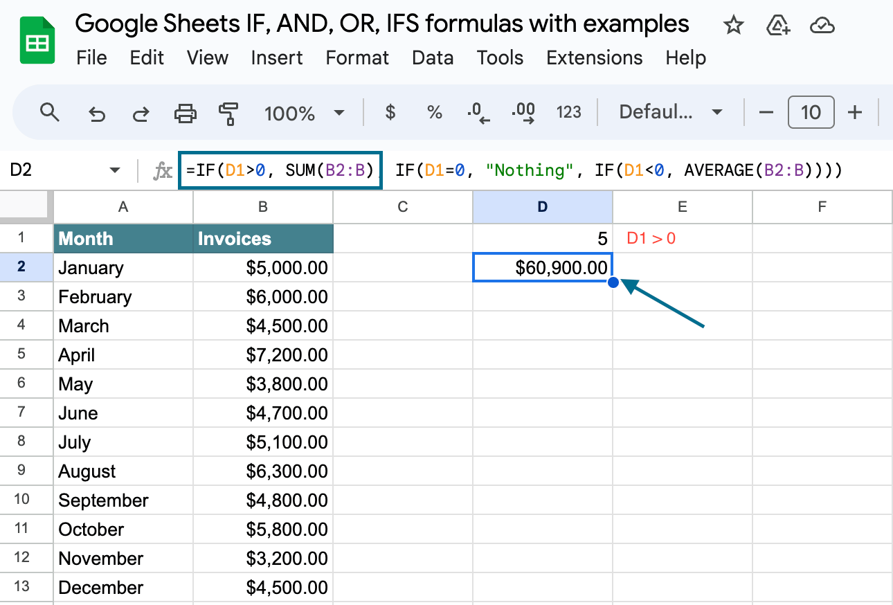
Interpretation of the nested IF Google Sheets formula:
If the value in the D1 cell is above zero (logical_expression#1), then the formula will return the sum of values in the range B2:B (value_if_true).
If the D1 cell is empty or its value is zero (logical_expression#2), then the formula will return “Nothing” (value_if_true).
If the value in the D1 cell is below zero (logical_expression#3), then the formula will return the average of values in the range B2:B (value_if_true).
Nested IF statements can be improved with other logical functions: AND and OR.
IF + AND/OR Google Sheets for multiple logical expressions
Google Sheets AND and OR function explained
| AND function | OR function | |
| Returns TRUE | If all of the provided logical expressions are logically true* | If any of the provided logical expressions is logically true |
| Returns FALSE | If any of the provided logical expressions is logically false | If all of the provided logical expressions are logically false |
| Syntax | =AND(logical_expression1, [logical_expression2, ...]) | =OR(logical_expression1, [logical_expression2, ...]) |
* All numbers (including negative ones) are logically true. The number 0 is logically false.
Let’s combine AND/OR with IF and check out how this works:
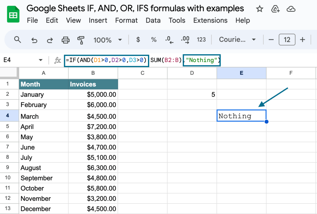
IF+AND Google Sheets formula example
=IF(AND(D1>0,D2>0,D3>0),SUM(B2:B),"Nothing")
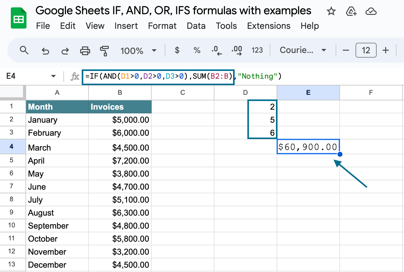
Interpretation of the IF AND Google Sheets formula:
If the values in the cells D1 (logical_expression#1), D2 (logical_expression#2), and D3 (logical_expression#3) are above zero, then the formula will return the sum of values in the range B2:B (value_if_true). Otherwise, if any of the logical expressions is false, the formula will return “Nothing” (value_if_false).
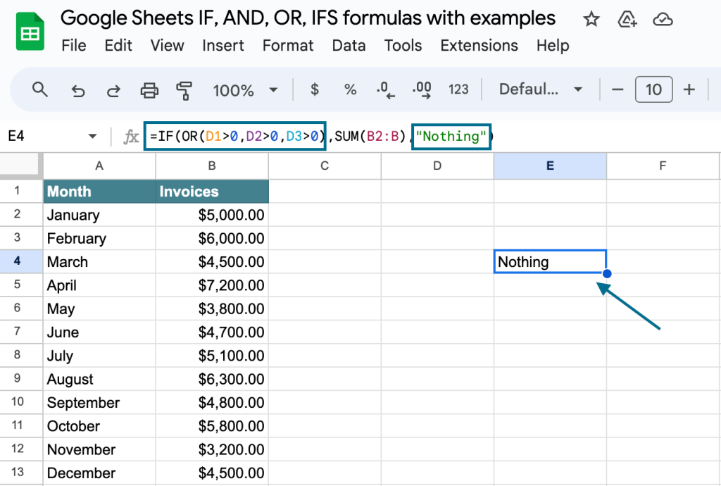
IF OR Google Sheets formula example
=IF(OR(D1>0,D2>0,D3>0),SUM(B2:B),"Nothing")
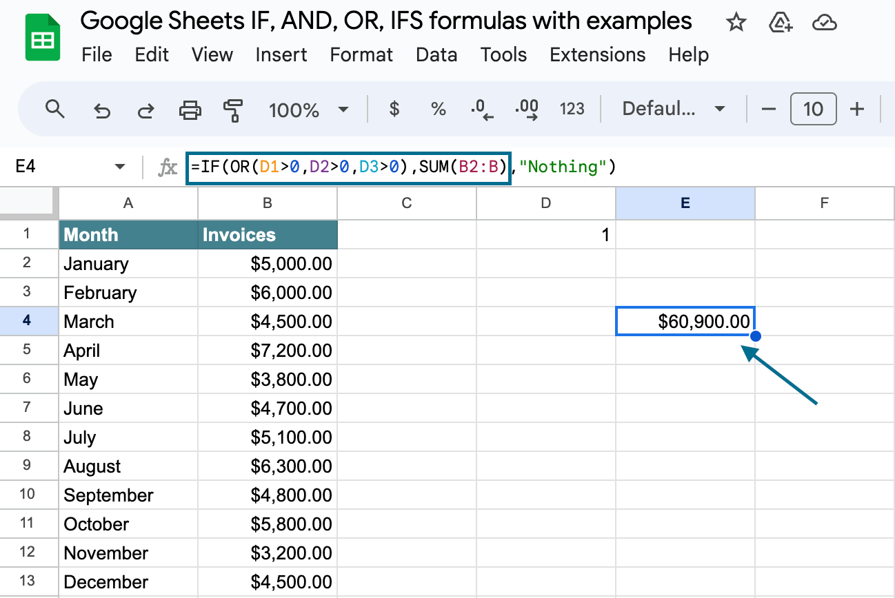
Interpretation of the IF OR Google Sheets formula:
If the value in the cell D1 (logical_expression#1), or D2 (logical_expression#2), or D3 (logical_expression#3) is above zero, then the formula will return the sum of values in the range B2:B (value_if_true). Otherwise, if all of the logical expressions are false, the IF OR Google Sheets formulawill return “Nothing” (value_if_false).
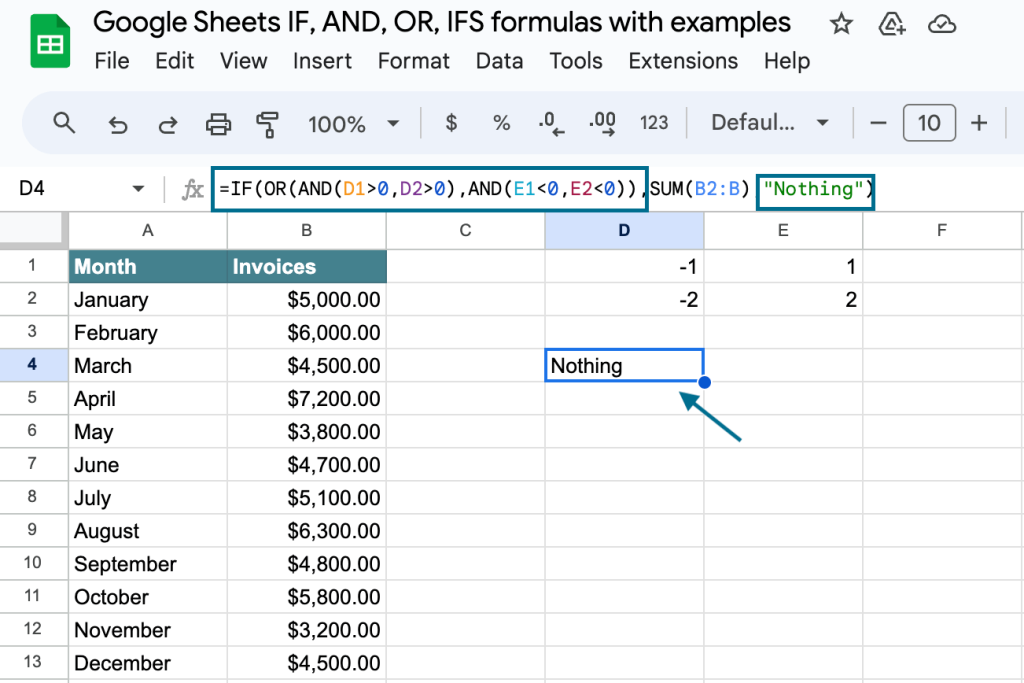
IF+AND+OR Google Sheets formula example
=IF(OR(AND(D1>0,D2>0),AND(E1<0,E2<0)),SUM(B2:B),"Nothing")
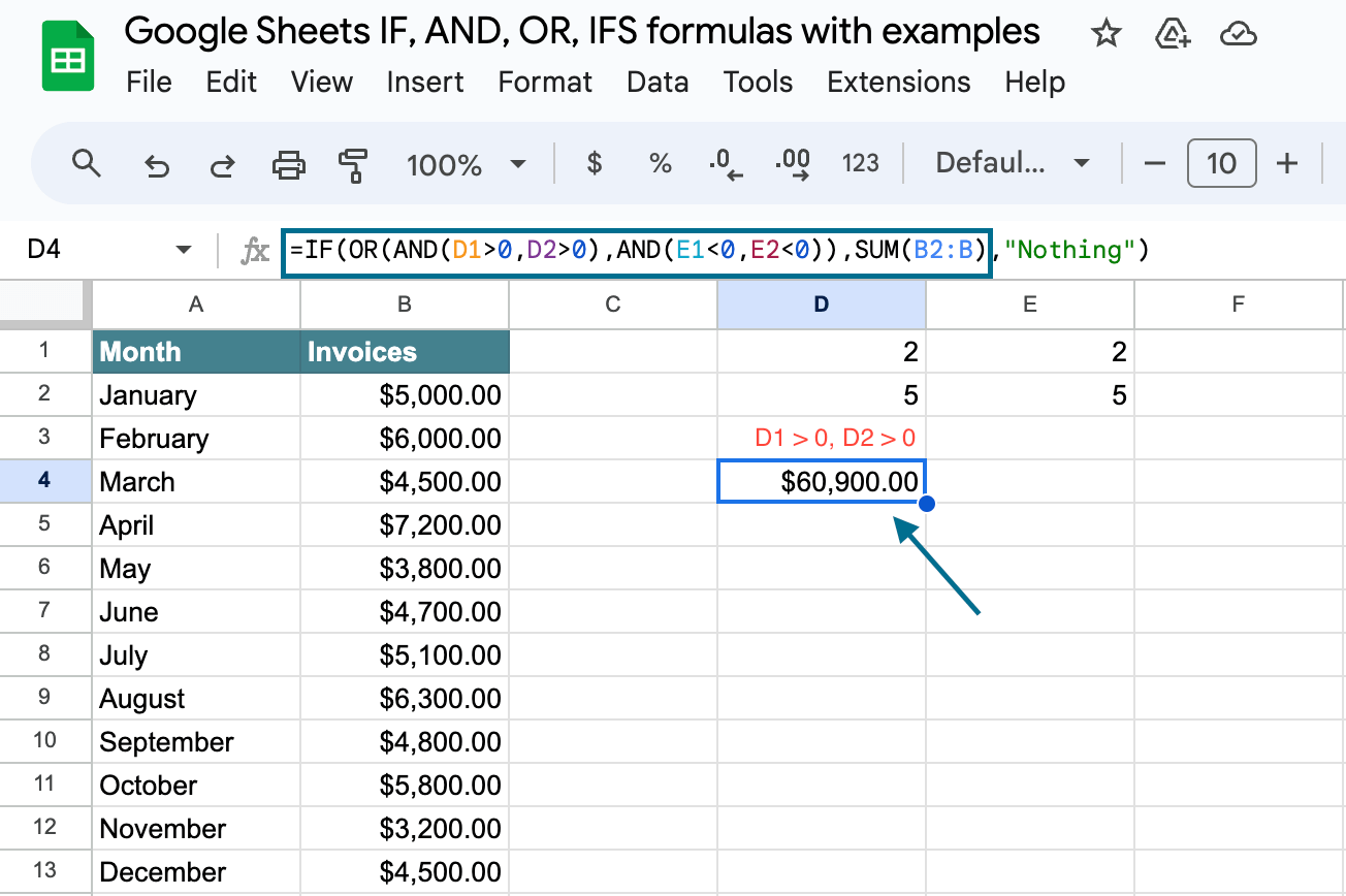
Interpretation of the IF AND OR Google Sheets formula:
If the values in cells D1 and D2 are above zero (logical_expression#1), or the values in cells E1 and E2 are below zero (logical_expression#2), then the formula will return the sum of values in the range B2:B (value_if_true). Otherwise, if all of the logical expressions are false, the formula will return “Nothing” (value_if_false).
Logical operators (AND and OR) let you include versatile conditions in your Google Sheets IF THEN formula. Keep in mind that AND/OR don’t work in arrays. Besides, multiple IF statements can be quite difficult to build and maintain. An alternative solution is to go with the IFS function.
IFS Google Sheets function explained
IFS Google Sheets syntax
=IFS(logical_expression#1, value_if_true, logical_expression#2, value_if_true, logical_expression#3, value_if_true,...)
IFS Google Sheets function evaluates multiple logical expressions and returns the first true value. If all the logical expressions are false, the function returns #N/A.
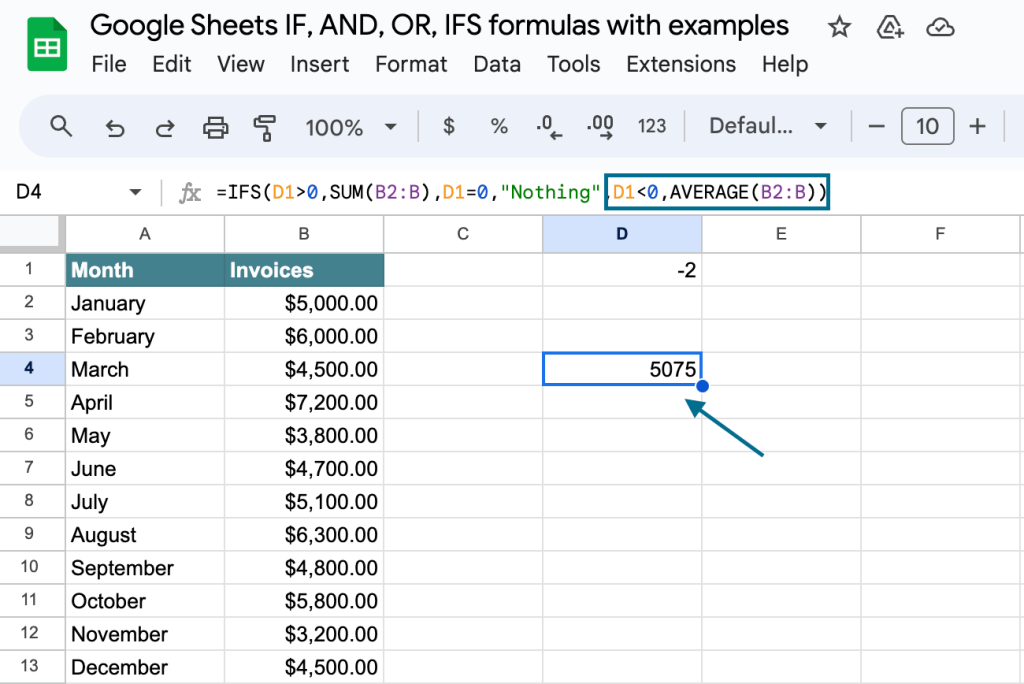
Google Sheets IFS formula example
=IFS(D1>0,SUM(B2:B),D1=0,"Nothing",D1<0,AVERAGE(B2:B))
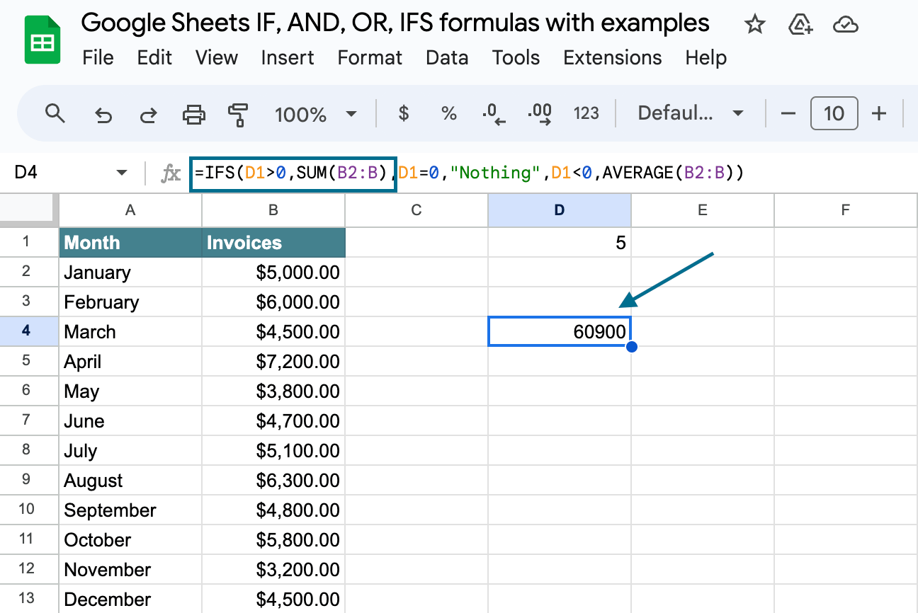
Interpretation of the IFS Google Sheets formula:
If the value in the D1 cell is above zero (logical_expression#1), then the formula will return the sum of values in the range B2:B (value_if_true).
If the D1 cell is empty or its value equals zero (logical_expression#2), then the formula will return “Nothing” (value_if_true).
If the value in the D1 cell is below zero (logical_expression#3), then the formula will return the average of values in the range B2:B (value_if_true).
IFS vs. multiple IF statements Google Sheets
| Nested IF formula |
=IF(logical_expression#1, value_if_true,IF(logical_expression#2, value_if_true,IF(logical_expression#3, value_if_true,value_if_false))) |
| IFS formula |
=IFS(logical_expression#1, value_if_true,logical_expression#2, value_if_true,logical_expression#3, value_if_true) |
The Google Sheets IFS function rests on true values only – it does not have value_if_false. But the major difference between IF and IFS can be revealed when dealing with arrays. Let’s explore this through an example.
IFS vs. nested IF statements example
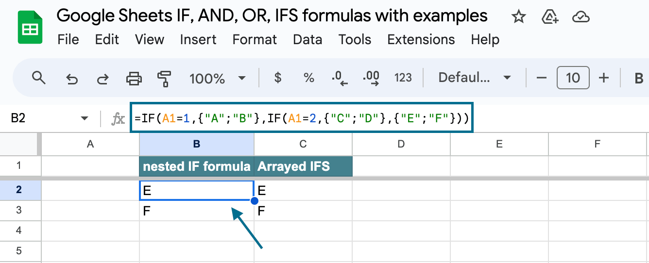
We have three logic expressions:
- if the value in the A1 cell equals 1, then show “A” and “B”
- if the value in the A1 cell equals 2, then show “C” and “D”
- if the A1 cell is empty, then show “E” and “F”.
The multiple IF statements Google Sheets formula will look like this:
=IF(A1=1,{"A";"B"},IF(A1=2,{"C";"D"},{"E";"F"}))
And that’s how it works in Google Sheets:
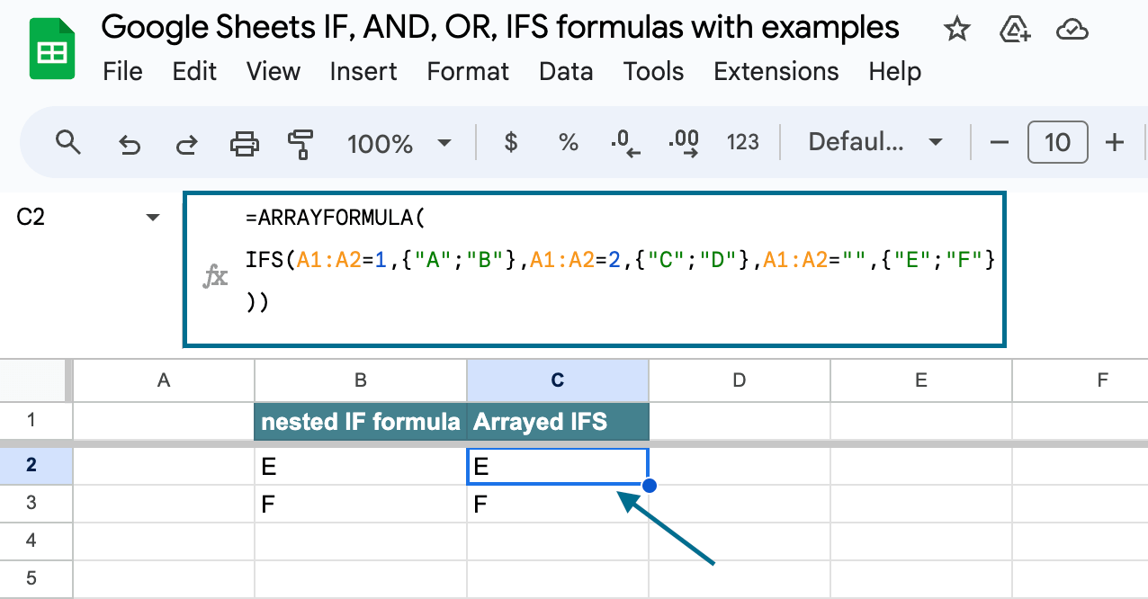
The Google Sheets IFS function returns a single-cell output and does not support arrayed output. To return an arrayed output, IFS expects an arrayed input, such as:
=ARRAYFORMULA(
    IFS(A1:A2=1, {"A";"B"}, A1:A2=2, {"C";"D"}, A1:A2="", {"E";"F"}
 )
In this case, however, the input range includes two cells: A1 and A2.
IF, AND, OR, IFS formula examples in real-life use cases
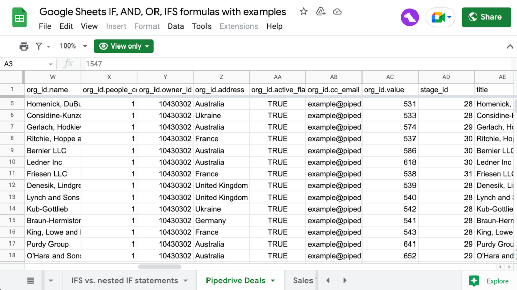
Now, let’s see how to understand your sales data better using IF, AND, OR, and IFS formulas. We use Pipedrive as our sales CRM software to store all our sales data. To implement these formulas on the dataset, we’ll be using a data automation solution, Coupler.io, to send data from Pipedrive to Google Sheets in 3 steps.
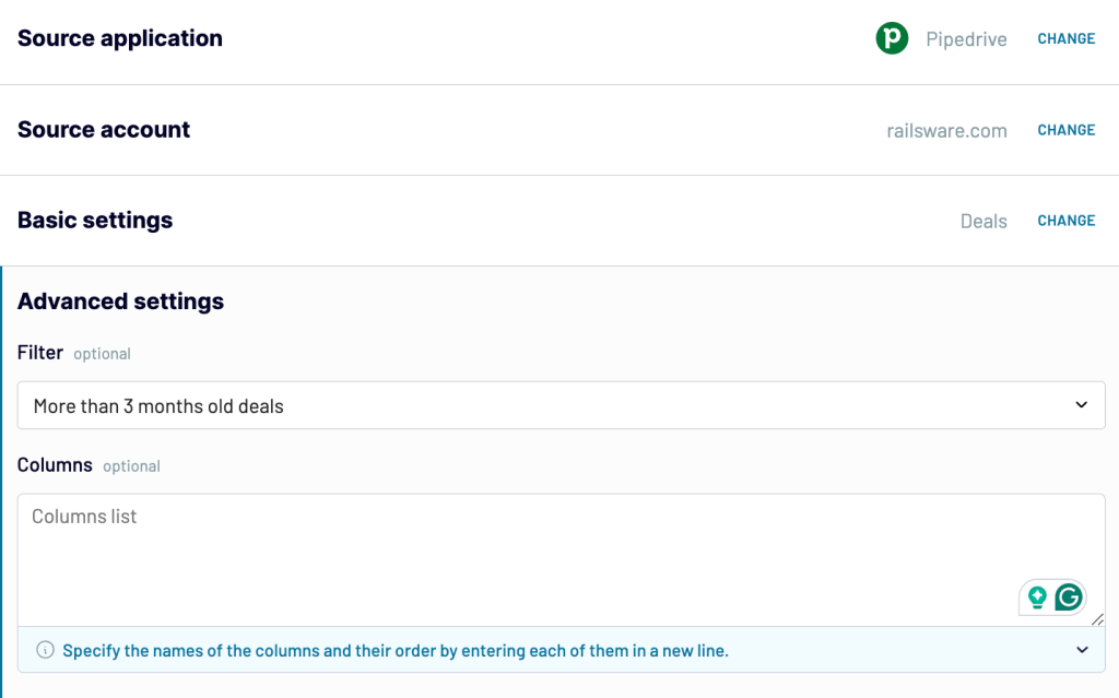
Step 1: Collect Pipedrive data
Click on Proceed in the form below.
Sign up to Coupler.io for free and connect your Pipedrive account. Select the data entity – deals. You can also set up advanced settings like selecting filtered datasets, and specific columns.
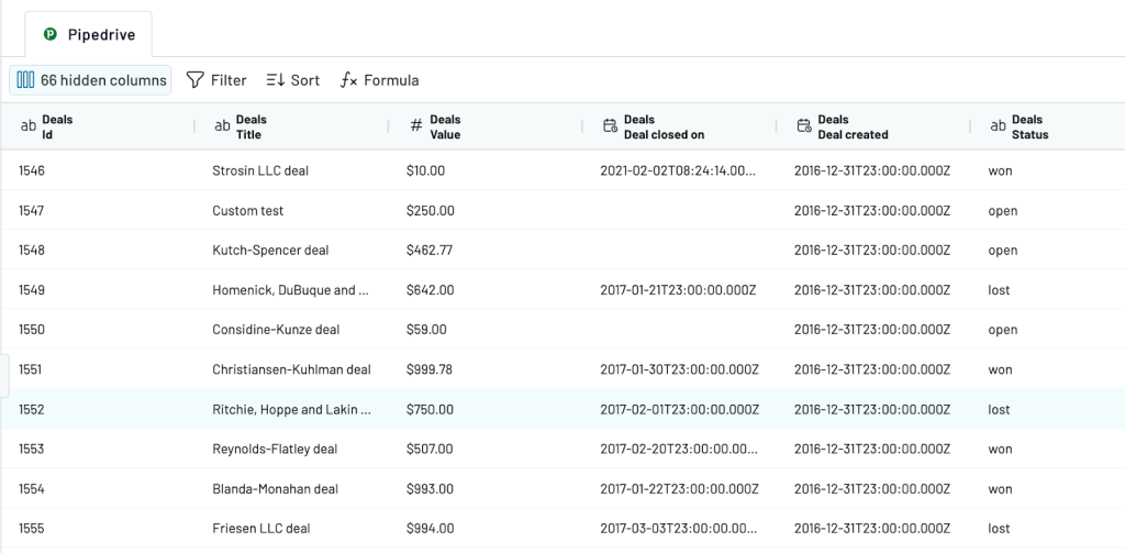
Step 2: Transform data
After you connect your applications, you can organize your sales data by filtering, sorting, adding new columns, and hiding unnecessary ones.
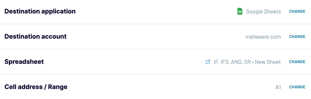
Select the spreadsheet file and sheet name in the destination settings to move this data to Google Sheets.
Step 3: Schedule updates
Toggle the ‘Automatic data refresh’ and set up the data update schedule to always have near real-time data in Google Sheets.
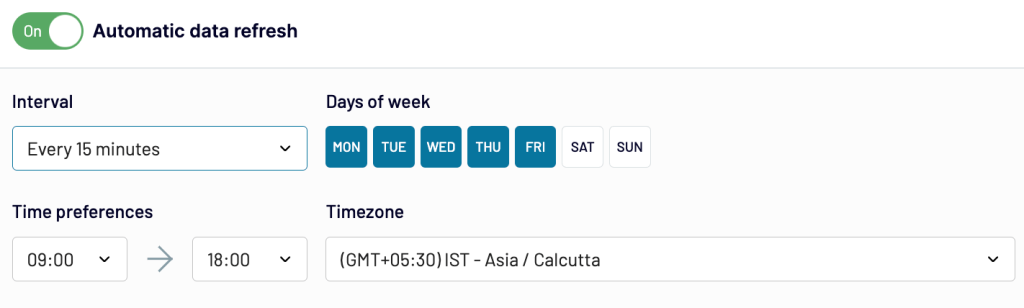
When the importer is scheduled, you’ll have updated, real-time, and analysis-ready data in Google Sheets.
Calculating sales metrics
Now, you have two options to calculate the sales metrics from the Pipedrive data.
- Create a sales dashboard in Google Sheets with IF and IFS formulas
- Use the Coupler.io importer
You’ll need to use long and complex formulas like nested IF and IFS to build this sales dashboard from scratch in Google Sheets.
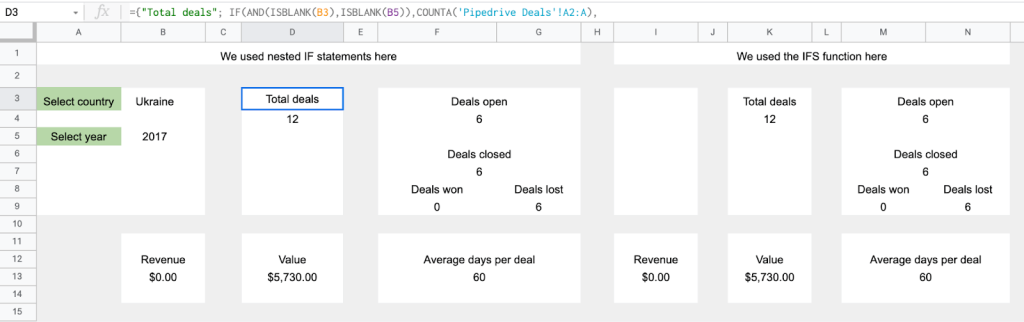
Here is an example of the formula for value metric in the sales dashboard using Nested IF and IFS.
Nested IF statements
={"Value";IF(AND(ISBLANK(B3), ISBLANK(B5)),SUM('Pipedrive Deals'!AF2:AF),<br><br>IF(ISBLANK(B5), SUM(IFERROR(<br>Filter('Pipedrive Deals'!AF2:AF,'Pipedrive Deals'!Z2:Z=B3))),<br><br>IF(ISBLANK(B3), SUM(IFERROR(<br>Filter('Pipedrive Deals'!AF2:AF,'Pipedrive Deals'!CN2:CN=B5))), SUM(IFERROR(<br>Filter('Pipedrive Deals'!AF2:AF,'Pipedrive Deals'!Z2:Z=B3,'Pipedrive Deals'!CN2:CN=B5))))))}<br>
IFS functions
={"Value";IFS(AND(ISBLANK(B3),ISBLANK(B5)),SUMIF('Pipedrive Deals'!AF2:AF),ISBLANK(B5),SUM(IFERROR(
Filter('Pipedrive Deals'!AF2:AF,'Pipedrive Deals'!Z2:Z=B3))),ISBLANK(B3),SUM(IFERROR(Filter('Pipedrive Deals'!AF2:AF,'Pipedrive Deals'!CN2:CN=B5))),AND(NOT(ISBLANK(B3)),NOT(ISBLANK(B5))),SUM(IFERROR(Filter('Pipedrive Deals'!AF2:AF,'Pipedrive Deals'!Z2:Z=B3,'Pipedrive Deals'!CN2:CN=B5))))}
Both formulas give accurate results. But With so many IF statements, it is hard to read, understand, and update the formula. It is easy to make mistakes, like missing a parenthesis or mixing up the order of operations. Moreover, these complex formulas can also slow down the spreadsheet.
The Coupler.io importer is a good alternative in this scenario. You can go to the ‘Transform data’ step and manipulate your data using the options below.
- Column management – Hide columns that are not required for analysis. Also, rename and rearrange columns as needed.
- Filter – Based on the deal status, filter lost or won deals.
- Sort – Organize your lost deals from highest to lowest based on value and vice versa.
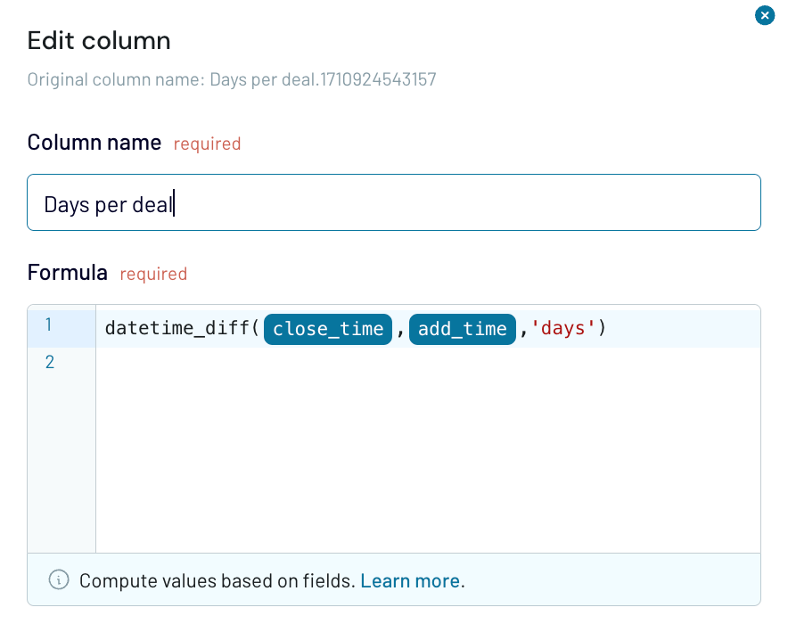
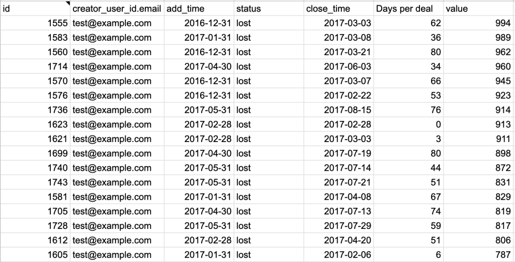
- Custom formulas – Create new columns by adding formulas to the existing columns. For example, you can calculate the days per each deal.
Now you have calculated sales metrics like value and days per deal without using complex Google Sheets formulas.
To take your sales analysis to the next level, connect your data to a sales overview dashboard template. Here, you can view key metrics like total revenue, deals won, and revenue per deal in real-time.
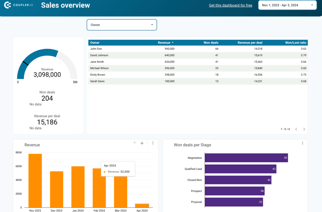
You can interpret the trends in revenue, open deals, open deals value, average days to close, and win/loss ratio. For example, in the above dashboard, ‘won deals per stage’ shows the sales pipeline health, where more deals are closed in the negotiation stage. By tracking and visualizing the lost reasons, it is easy to train the team and improve efforts.
To get this dashboard with your sales data, click ‘Get Dashboard for free’ and follow the instructions in the readme tab.
IFS or nested IF statements in Google Sheets – which are better?
Within this example, we can speculate that IFS is just a shorthand for nested IF statements. But that’s not the fundamental truth, since each use case has its own requirements. Anyway, now you know what you can do with IF and IFS, as well as logical operators AND and OR. And don’t forget about Coupler.io, which can simplify and automate data import to Google Sheets and Excel. Enjoy your data and good luck!