Let’s imagine a situation where you’ve got 2 columns in a Google spreadsheet: the 1st with prices, the 2nd with the number of items, and you need to multiply them in the 3rd column. What do you usually do in this case? If you were like me in the past, you’d compose a formula in the first row and copy-paste it into the other rows. A good old-school method that works fine.
But what if there are 1000 rows or even more? Annoying, right? Let alone time-consuming. It can also cause a performance issue since a bunch of similar formulas slow down the whole spreadsheet. And, if you need to add a new value and create a separate row for it, Google Sheets will not automatically copy the formula. OK, so what’s the solution here?
Actually, there is a dynamic and efficient way to address the discussed issues, and this way is called ARRAYFORMULA. In this article, we’ll explain how you can use it and cover a few cases. If you prefer watching to reading, check out this video tutorial about ARRAYFORMULA in Google Sheets.
What is ARRAYFORMULA in Google Sheets?
In short, ARRAYFORMULA is a function that outputs a range of cells instead of just a single value and can be used with non-array functions.
According to Google Sheets documentation, ARRAYFORMULA enables
“the display of values returned from an array formula into multiple rows and/or columns and the use of non-array functions with arrays”.
Well, the definition kills any desire to use the function, but wait, do not jump to a conclusion. It is tremendously useful and easier to use than it sounds in the description.
To use it in Google Sheets, you can either directly type “ARRAYFORMULA” or hit a Ctrl+Shift+Enter Google Sheets shortcut (Cmd + Shift + Enter on a Mac), while your cursor is in the formula bar to make a formula an array formula (Google Sheets will automatically add ARRAYFORMULA to the start of the formula).
How does Google Sheets ARRAYFORMULA solve the problems?
- Since this is one single formula even for a huge dataset, you won’t end up with a lot of formulas, and your Google Sheets will run smoothly.
- ARRAYFORMULA is also expandable – a change in one place will expand down the entire data range.
- And it is dynamic as well. When a new row is introduced into the dataset, the formula will automatically be applied to it.
Google Sheets ARRAYFORMULA syntax
=ARRAYFORMULA(array_formula)array_formula is a parameter that can be
- a range
- a mathematical expression using ranges of the same size, or
- a function that returns a result greater than one cell
Google Sheets ARRAYFORMULA example
Let’s have a closer look at how the ARRAYFORMULA works. The easiest way to understand this is through an example.
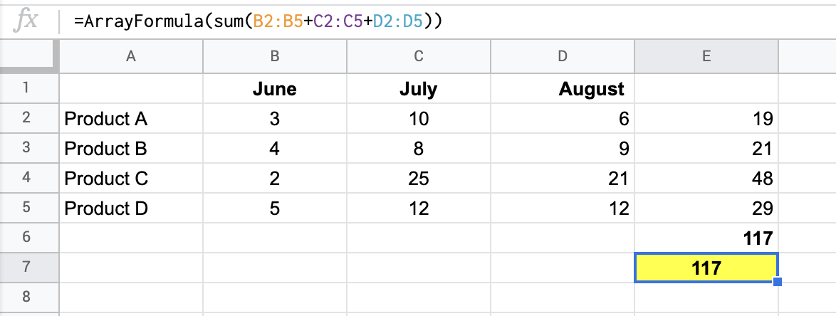
Let’s say we have a dataset showing the quantity of four different products sold in the summer months
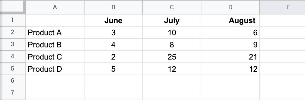
and we need to calculate the total amount of sold products.
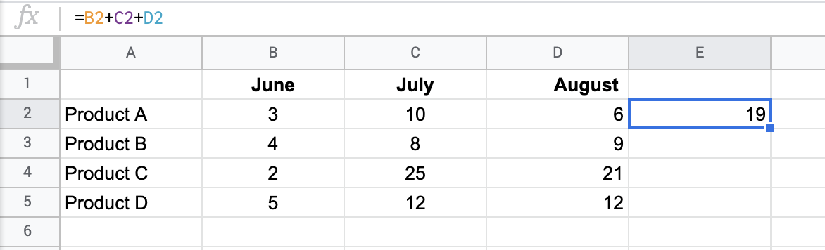
Sure, we could do it by writing a formula in column E that adds B, C, and D.
=B2+C2+D2
Or use the SUM function.
To find the sold quantity of B, C, and D products, you can copy the formula in E2 and then paste it into the cells E3, E4, and E5
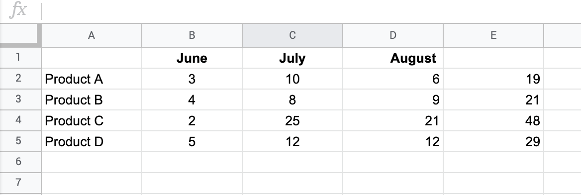
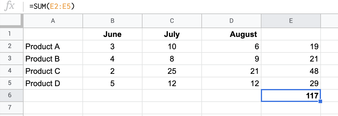
and then use SUM at the bottom of column E.
=sum(E2:E5)
However, the ARRAYFORMULA function lets you skip all those steps and get straight to the answer with a single formula, which saves you time and energy if you’ve got 1000+ products.
In our case we will have
=ArrayFormula(
   sum(B2:B5+C2:C5+D2:D5)
)
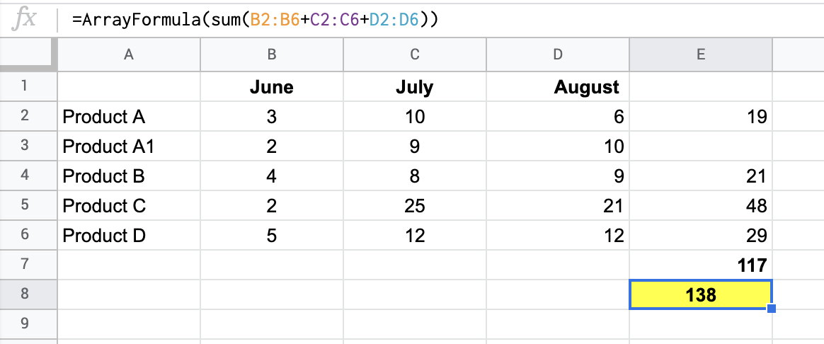
Now, I am adding a new range for Product A1.
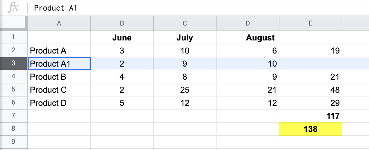
ARRAYFORMULA takes into account the new range (changes B5 to B6, C5 to C6, D5 to D6 in the formula), and does the calculation, unlike SUM, which is expected for Google Sheets. Now the formula looks as follows:
=ArrayFormula(
   sum(B2:B6+C2:C6+D2:D6)
)
ARRAYFORMULA with different Google Sheets functions
If a formula already returns an array of values, wrapping it up with ARRAYFORMULA is not necessary. This means that combining ARRAYFORMULA with, for example, FILTER, SEQUENCE, or QUERY, won’t bring any value.
At the same time, you cannot benefit from nesting ARRAYFORMULA with many non-array functions including:
- SUM
- SUMIFS
- COUNT
- COUNTA
- COUNTIFS
- CONCATENATE
- JOIN
- TEXTJOIN
- etc.
However, as we mentioned before, ARRAYFORMULA can be used with non-array functions, for example, IF, SUMIF, COUNTIF, VLOOKUP, and others.
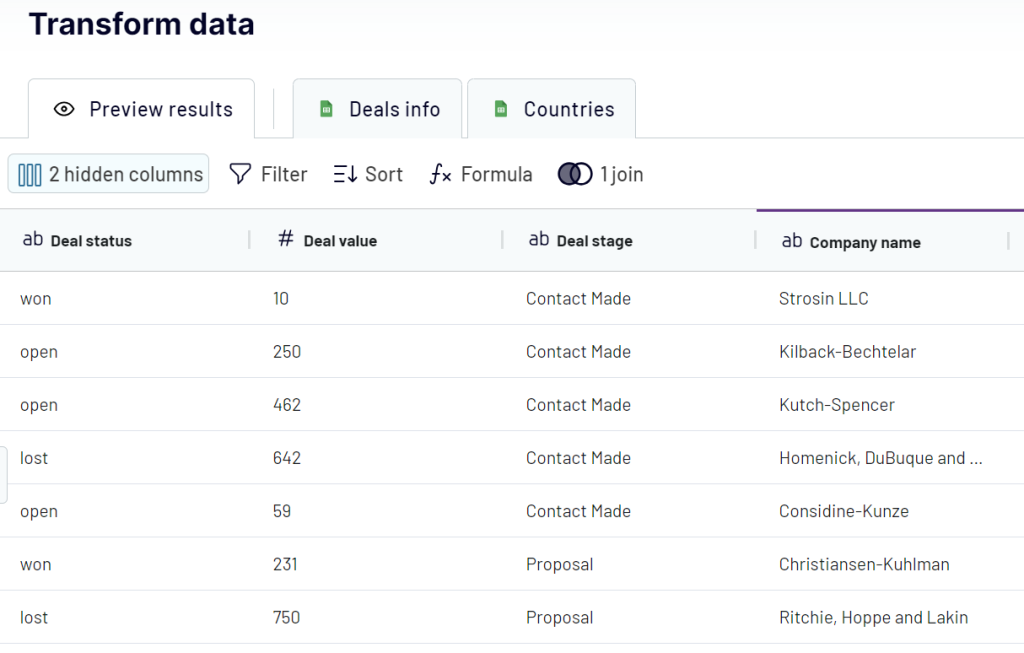
We’ll check out how they work below, but first, let’s get some datasets that we can use as examples. No need to copy and paste data since it’s not efficient and time-consuming. Instead, we can use Coupler.io, a reporting automation solution to automate exports from 50+ sources to Google Sheets. All you have to do is select the needed source and click Proceed in the form below. You can sign up for free with your Google account.
Once you connect your apps, you can filter, sort, add, and hide columns to organize your data.
Next, configure a data refresh schedule as you like. Taking this step, you’ll get ever-updating, real-time data in Google Sheets for your analytics purposes.
Google Sheets ARRAYFORMULA with IF function
To remind you, the IF function in Google Sheets works by performing a logical test that can only have one of two outcomes: true or false. Read more about IF and other logical functions in Google Sheets,
Let’s see how to use the IF function and ARRAY on the sales spreadsheet. Consider a standard IF statement that checks whether there are enough (more than 10) items left in stock for next month.
In cell G2, I’d like to display the text “order” if there are fewer than ten items left in stock, and “no” if the outcome is false.
=if(C2<10, "order", "no")
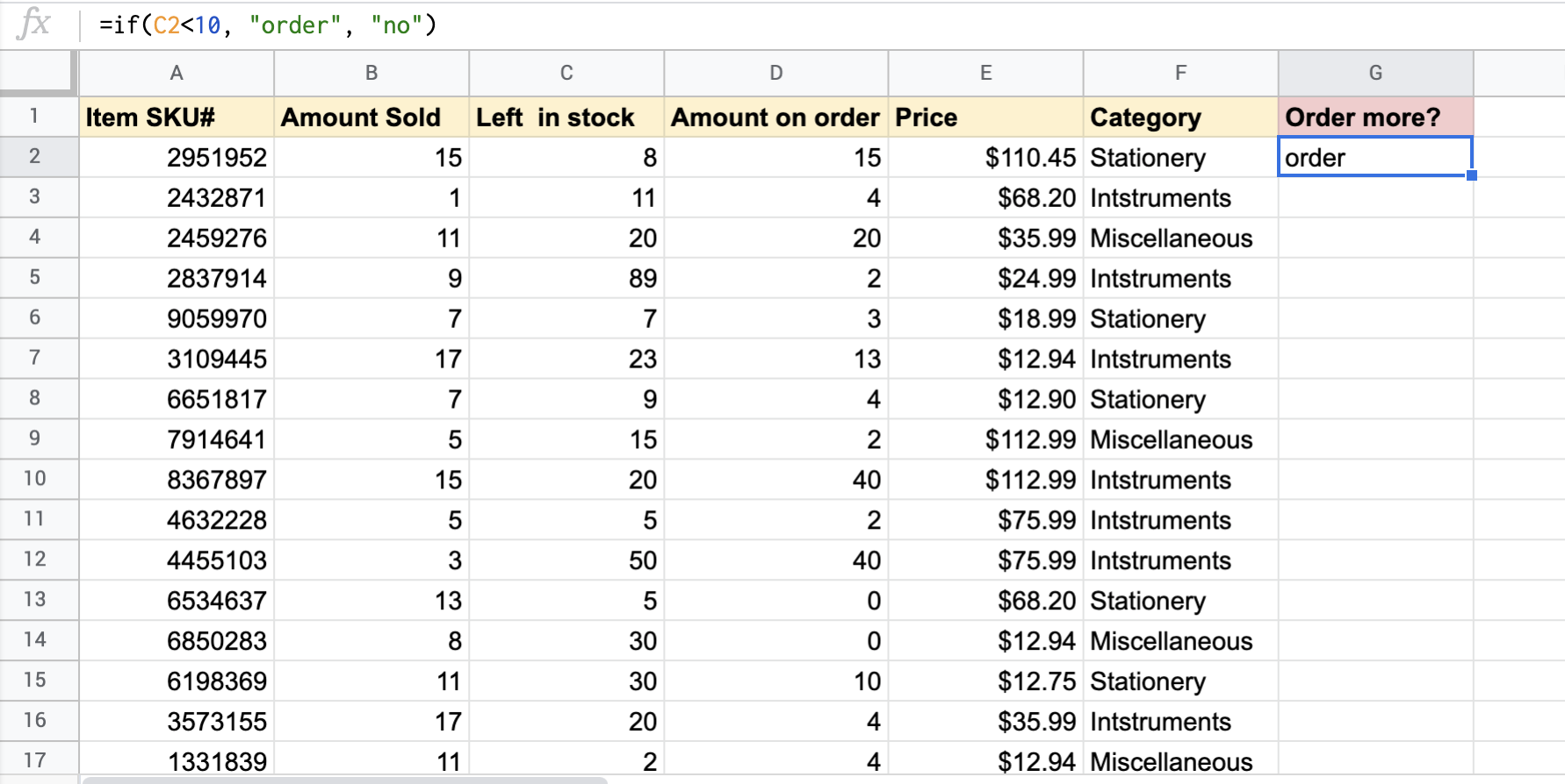
The IF function does its calculation and, for this first item, since there are only eight left in stock, the text “order” is displayed.
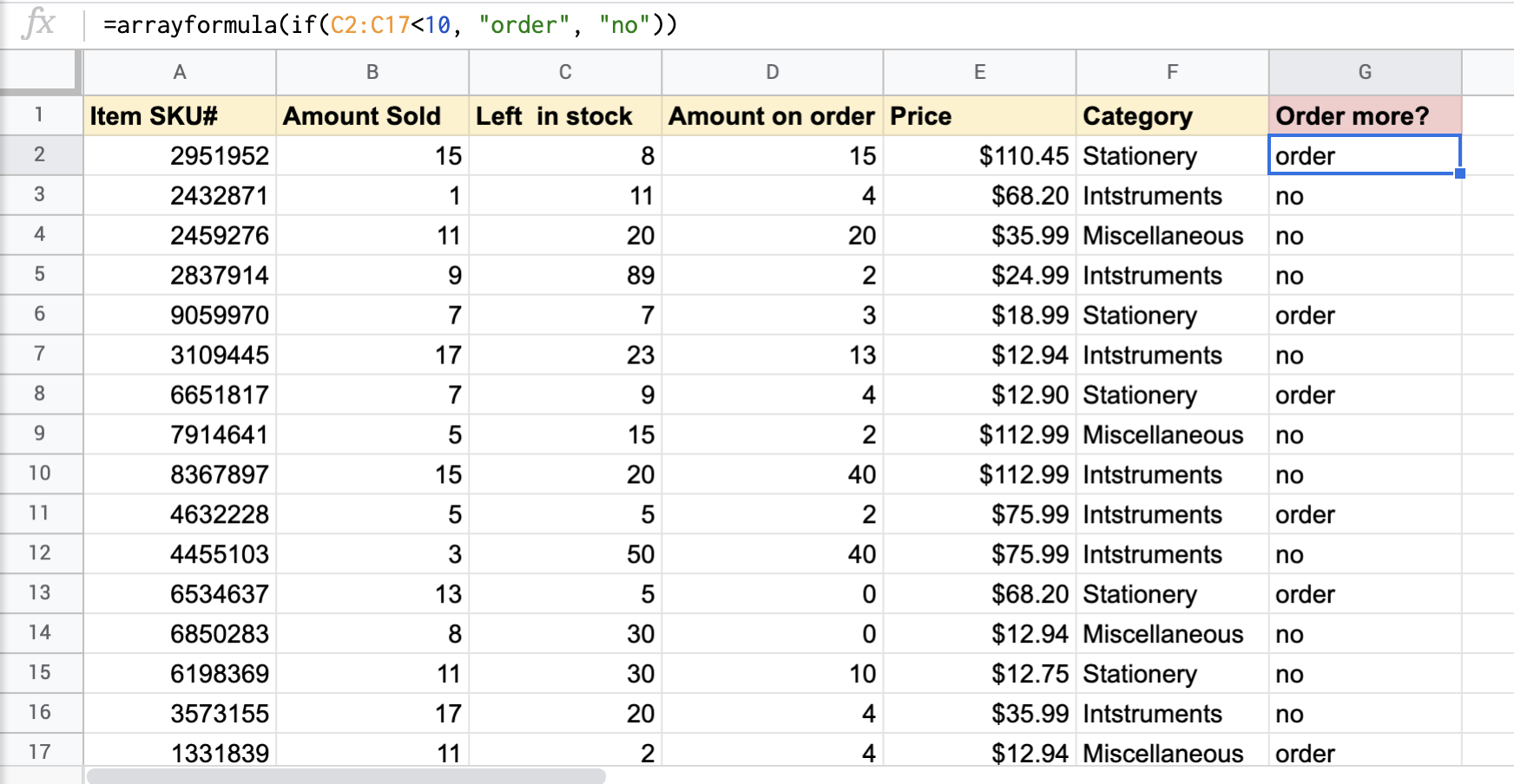
Now let’s run the test for each item, and this is where a single ARRAYFORMULA comes in handy. Type ARRAYFORMULA before IF, and it runs the IF statement across all the rows at once. Cool, right?
=arrayformula(
   if(C2:C17<10, "order", "no")
)
SUMIF & SUMIFS with ARRAYFORMULA in Google Sheets
Building on the previous example, let’s have a look at how ARRAYFORMULA can be used with SUMIF and SUMIFS Google Sheet functions.
SUMIF and SUMIFS are two independent functions in Google Sheets. SUMIF is used for adding values based on one condition and the purpose of SUMIFS is to sum the values in a range, based on multiple conditions.
SUMIF + ARRAYFORMULA in Google Sheets
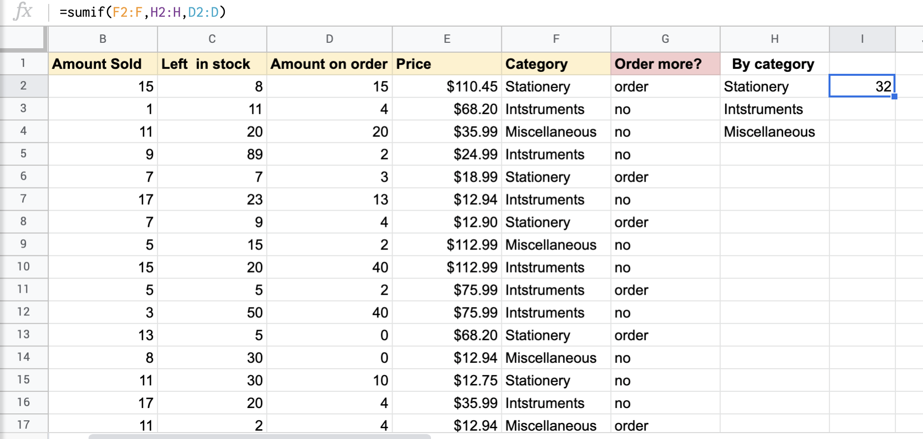
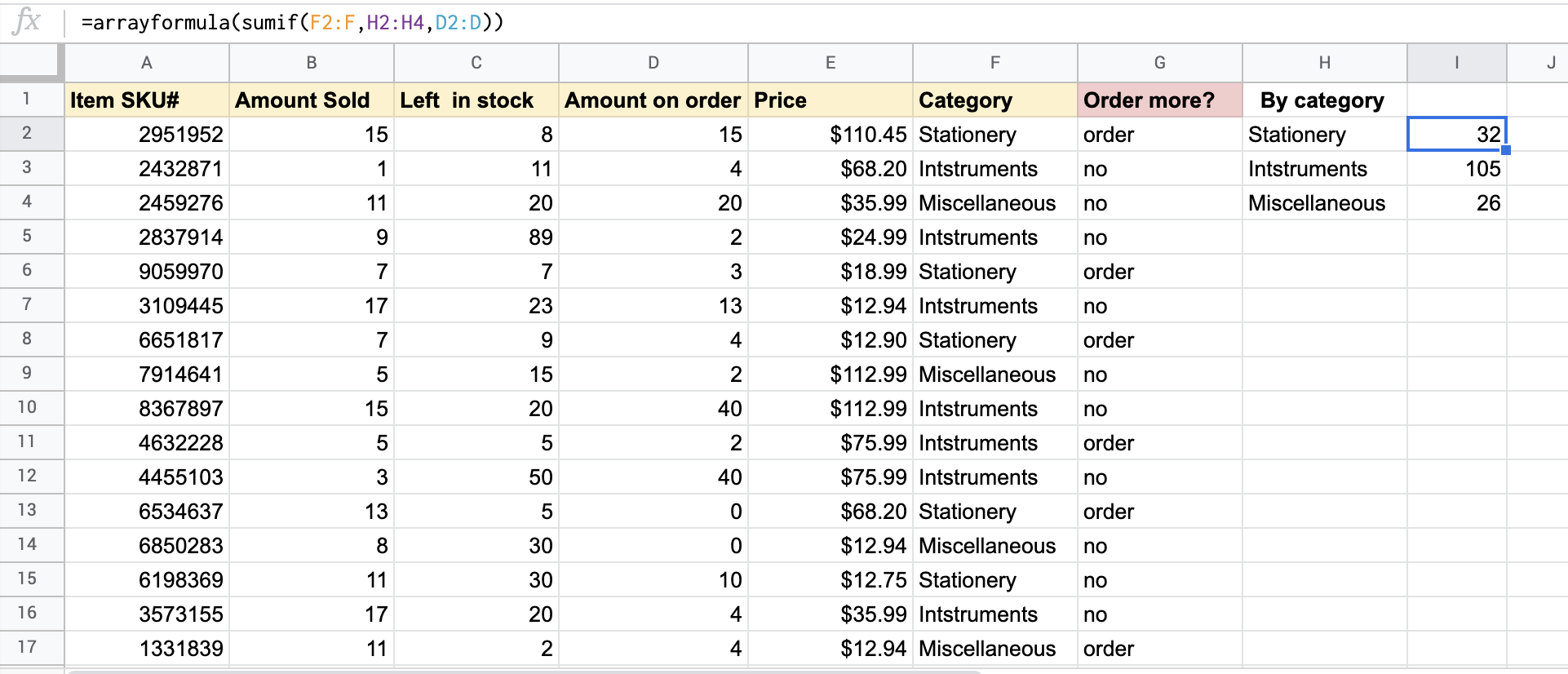
So, let’s code an array formula for SUMIF. Let’s say you need to find out how many stationery items have been already ordered and you apply SUMIF function, which returns you 32 in cell I2.
=sumif(F2:F,H2:H,D2:D)
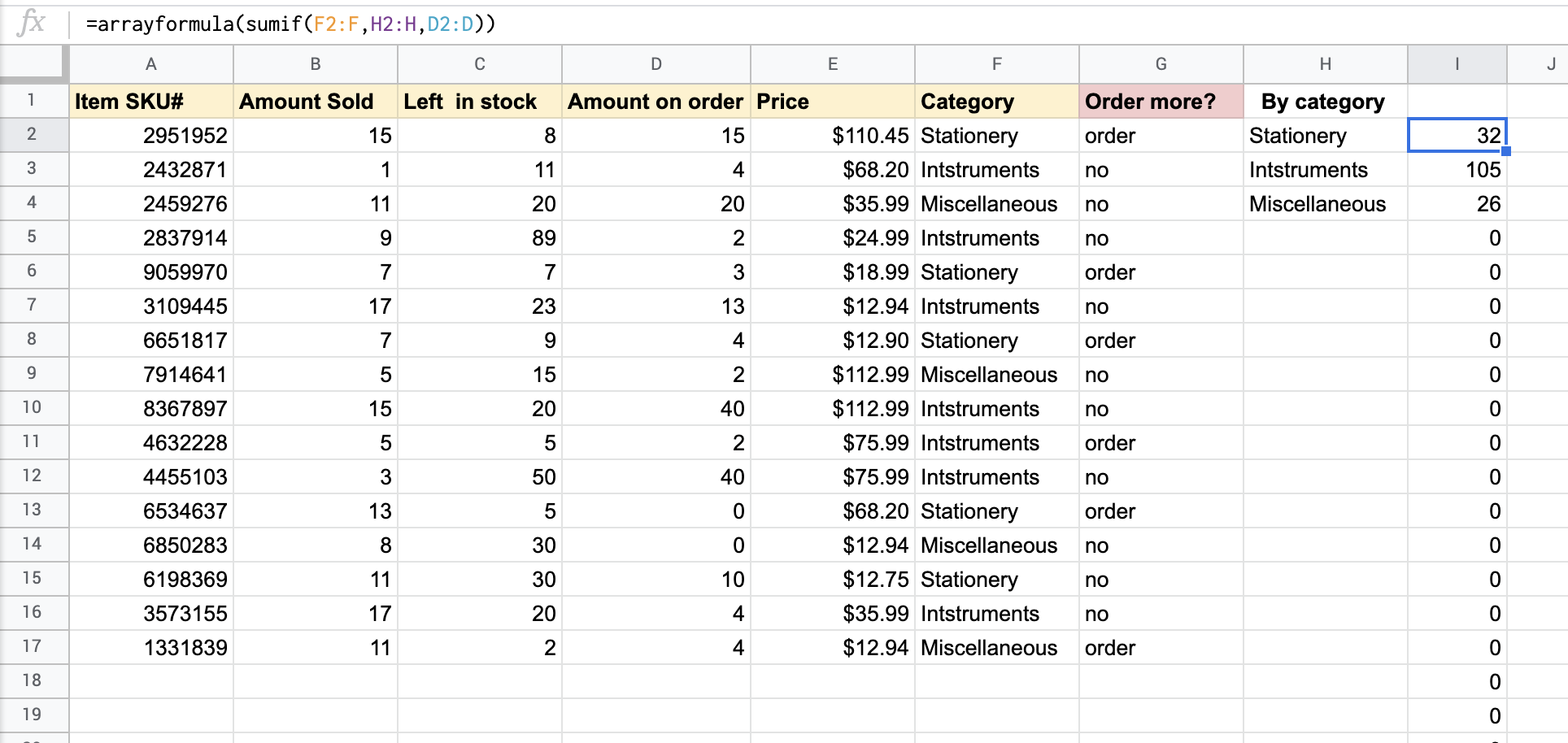
And if you want to know the number of items already ordered for each category, the best way is to apply ARRAYFORMULA, which again will be extremely helpful if you have way too many categories.
=arrayformula(
   sumif(F2:F,H2:H,D2:D)
)
SUMIFS + ARRAYFORMULA Google Sheets does not expand
With SUMIFS, things are a little bit more complicated. Its syntax is:
=SUMIFS(sum_range, range1, criteria1, [range2], [criteria2], ...)Unlike SUMIF, the SUMIFS function does not expand the results even if you use ARRAYFORMULA with it. The logic is simple, since SUMIFS in Google Sheets returns the sum of an array conditionally, so it can be nothing but a single result.
Let’s check it out.
=sumifs(D2:D17,F2:F17,H2:H4,G2:G17,I2:I4)
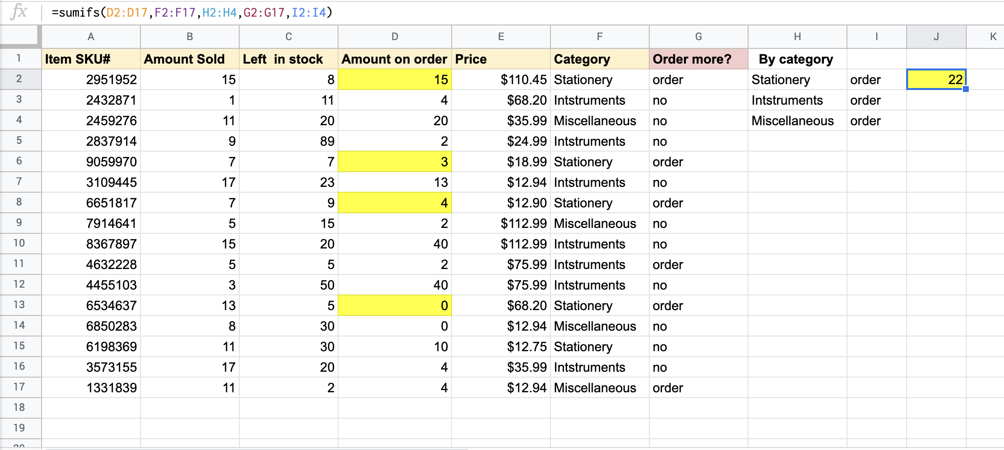
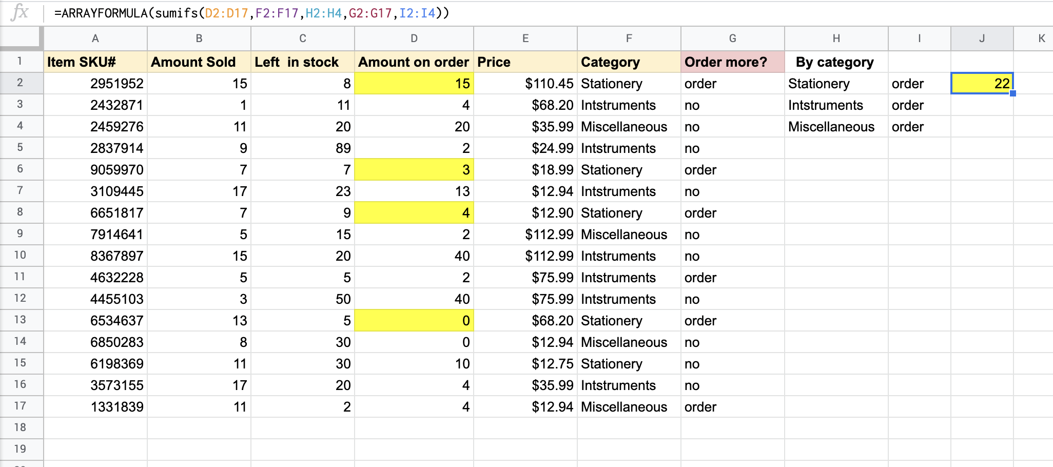
The SUMIFS in the above example sums up the amount of “Stationery” items that need to be ordered. And, even if we nest SUMIFS with ARRAYFORMULA, it won’t expand but will return a single result one way or another.
=ArrayFormula(
   sumifs(D2:D17,F2:F17,H2:H4,G2:G17,I2:I4)
)
To solve this expanding issue, one should use alternative formulas. There are several options on how to address SUMIFS-ARRAYFORMULA-expansion issues, and the easiest one is with the help of SUMIF.
Alternative #1: Google Sheets ARRAYFORMULA and SUMIF
Actually, the SUMIF function can handle multiple criteria to expand the results, though in a slightly tricky way. The main tip here is to combine ranges and corresponding criteria using AMPERSAND (&).
=ArrayFormula(
   sumif(F2:F17&G2:G17,H2:H4&I2:I4,D2:D17)
)
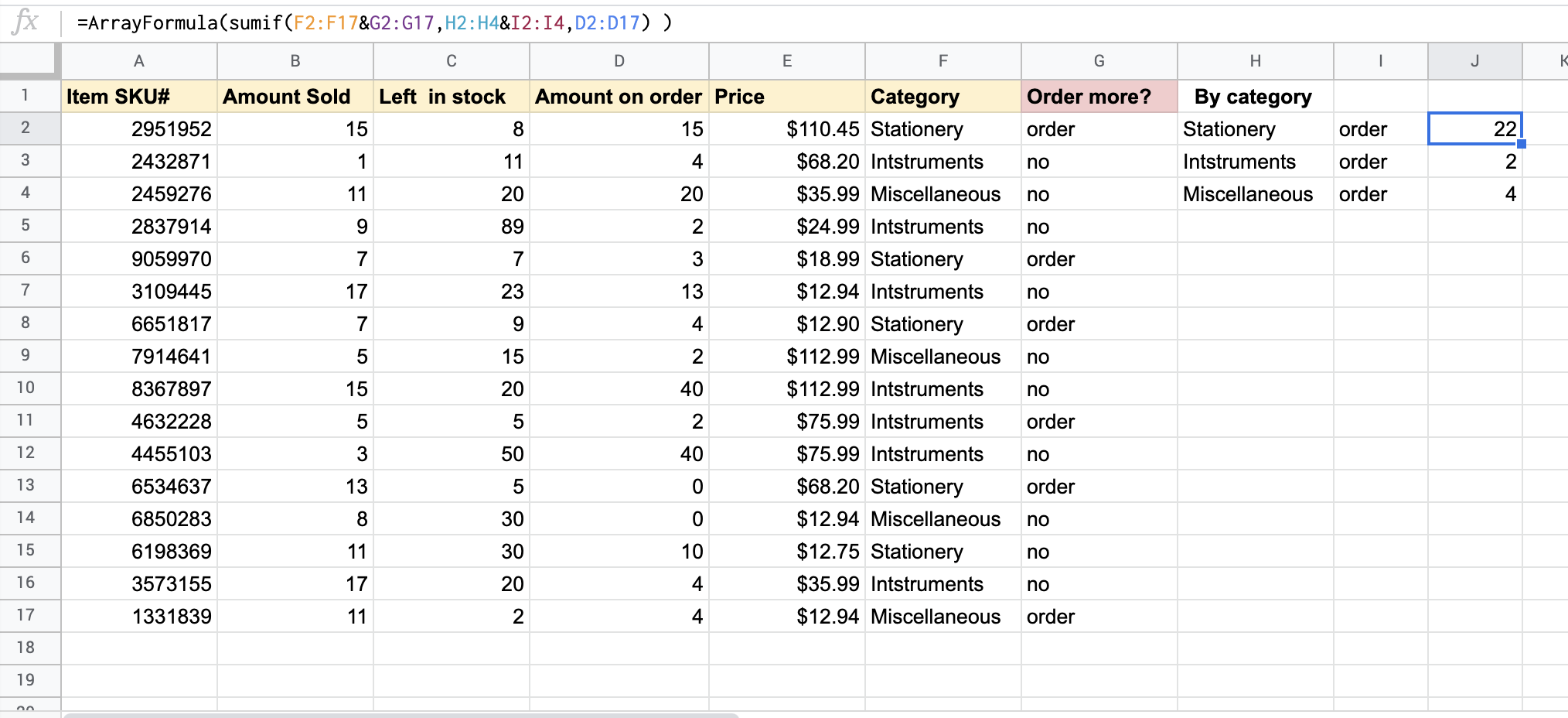
And, as you can see, it is perfectly expandable.
Alternative #2: Google Sheets ARRAYFORMULA, IF, LEN, VLOOKUP, QUERY
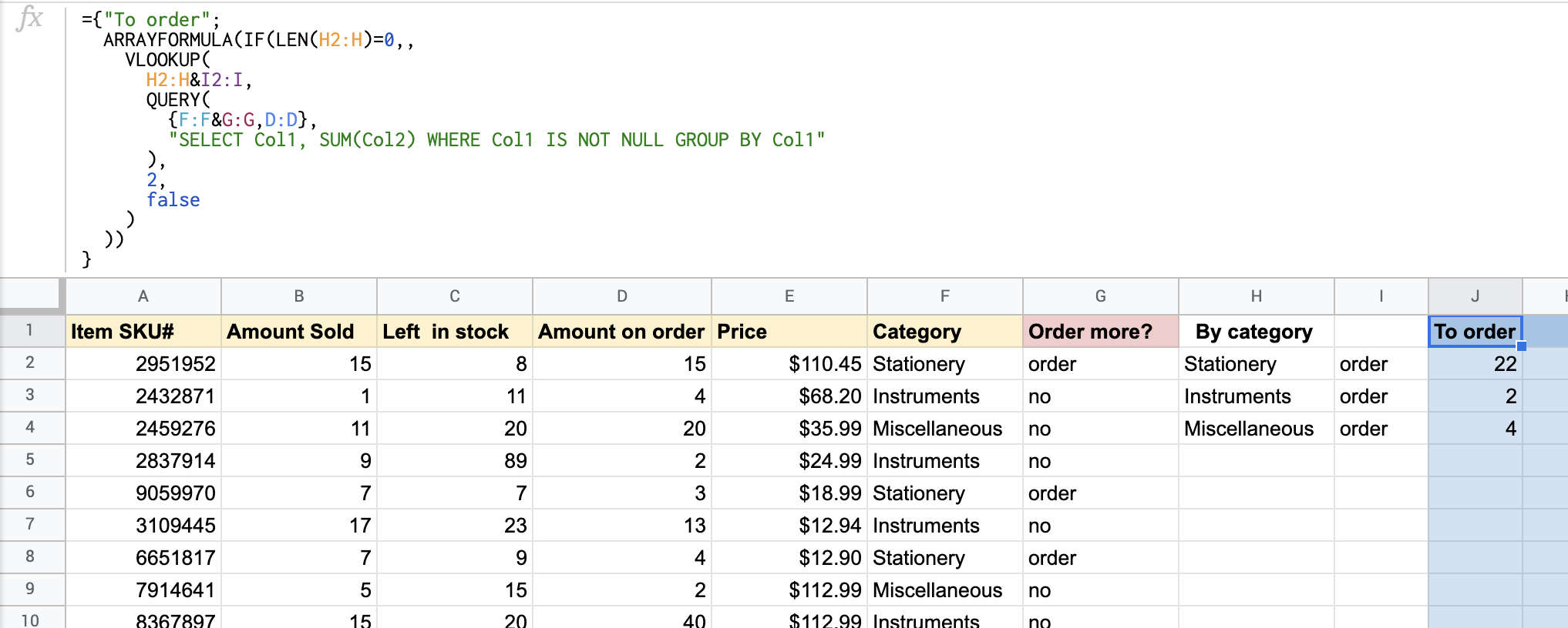
Another workaround is to use the combination of ARRAYFORMULA, IF, LEN, VLOOKUP, and QUERY functions. Looks complicated? Well, actually, it is. But the formula works perfectly, no doubt.
={"To order";
  ARRAYFORMULA(IF(LEN(H2:H)=0,,
    VLOOKUP(
      H2:H&I2:I,
      QUERY(
        {F:F&G:G,D:D},
        "SELECT Col1, SUM(Col2) WHERE Col1 IS NOT NULL GROUP BY Col1"
      ),
      2,
      false
    )
  ))
}
Can I use QUERY as an alternative to SUMIFS+ARRAYFORMULA in Google Sheets?
You may come up with the idea of trying to use something simpler, like QUERY solo, as some other internet resources suggest. Well, we tried to apply the following formula:
=query(A2:G,"Select sum(D) where F='"&H2&"'and G='"&I2&"' or F='"&H3&"'and G='"&I3&"' or F='"&H4&"'and G='"&I4&"' group by F,G label sum(D)''")
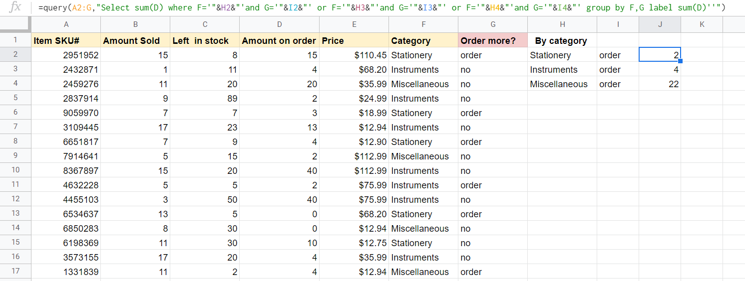
And logically it should have worked, but it hasn’t as it returns results in random order, which is not user-friendly at all, to say the least. So, if you have no prejudices or limitations about using SUMIF, better check out the Alternative #1.
Read more about the power of QUERY function in Google Sheets.
VLOOKUP and ARRAYFORMULA in Google Sheets
For a lot of Google sheets users, mastering VLOOKUP is the turning point. That’s when they are really getting comfortable with many functions and their application.
And, if you still haven’t mastered it, open up VLOOKUP by reading our dedicated post VLOOKUP Explained: How to Search Data Vertically in Spreadsheets.
Case 1. Vlookup+Arrayformula Google Sheets with multiple lookup criteria
As you are probably aware, the main limiting problem with VLOOKUP is that it only allows you to look for a single value. However, the real world often requires you to use two or more criteria when looking up data from a database. To vertically lookup multiple criteria, nest VLOOKUP with ARRAYFORMULA:
=ARRAYFORMULA(VLOOKUP({search-key#1;search-key#2;...}, range, column-index,[sorted/not-sorted])Let’s have a look at the already-familiar table, assuming we want to search for Item SKU# and return Amount Sold, Price and Category.
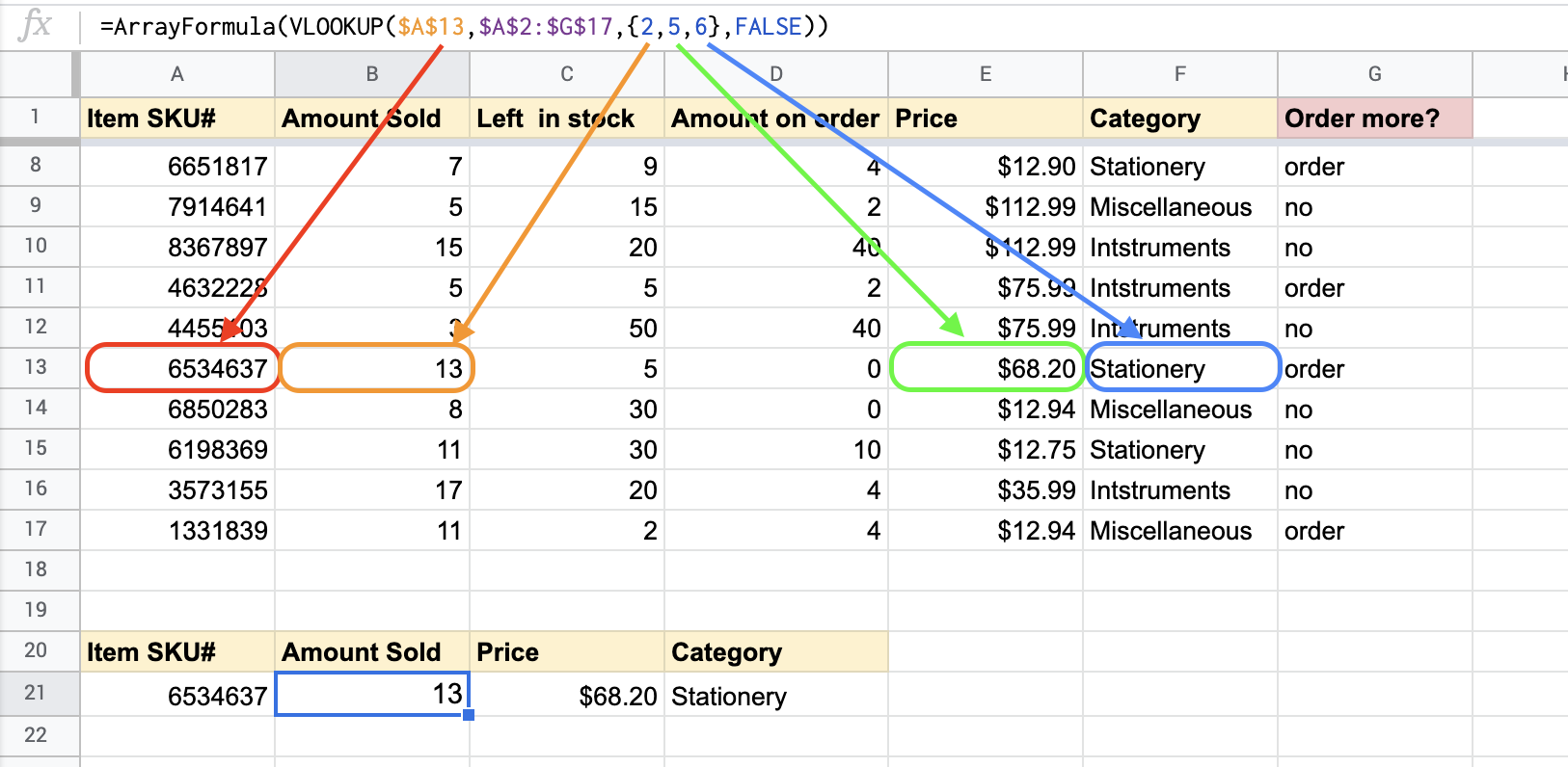
Since we need VLOOKUP to return multiple columns, let’s use curly brackets “{}” to indicate the columns we want to return, and apply ARRAYFORMULA, so Google Sheets knows we’re working with a range output, not a single value. My data table is in the range A2:G17 and the search value is in A13, so the formula will be as follows:
=ArrayFormula(
   vlookup($A$13,$A$2:$G$17,{2,5,6},FALSE)
)
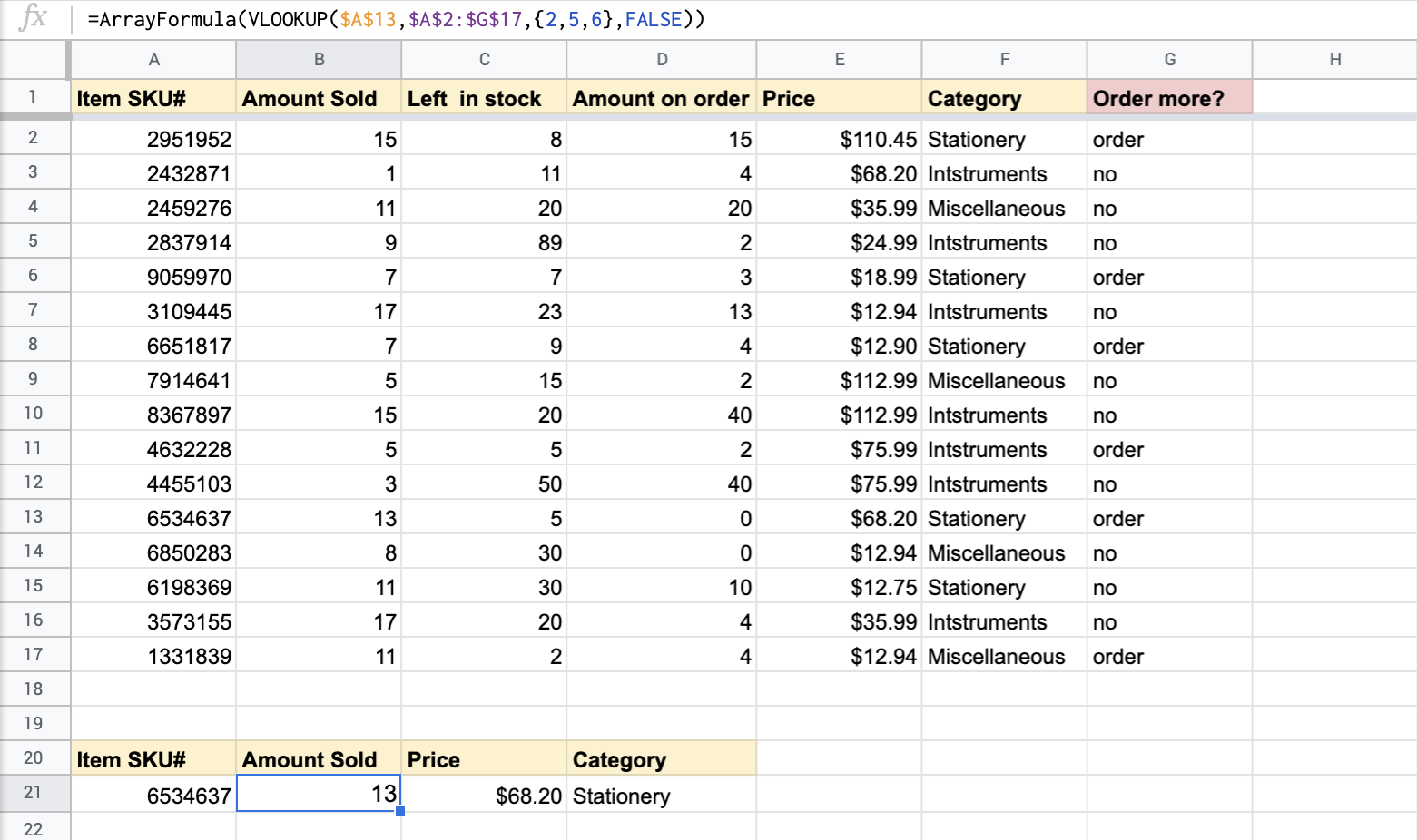
In fact, this is a regular VLOOKUP formula but, instead of a single column, we use an array of columns in curly brackets: {2,5,6}
Case 2. VLOOKUP and ARRAYFORMULA Google Sheets for vertical lookup
A more traditional use case of VLOOKUP and ARRAYFORMULA in Google Sheets is a vertical lookup.
With the help of Pipedrive to Google Sheets integration by Coupler.io, we have two sheets. The first one, Countries, contains two columns: Countries and Company name.
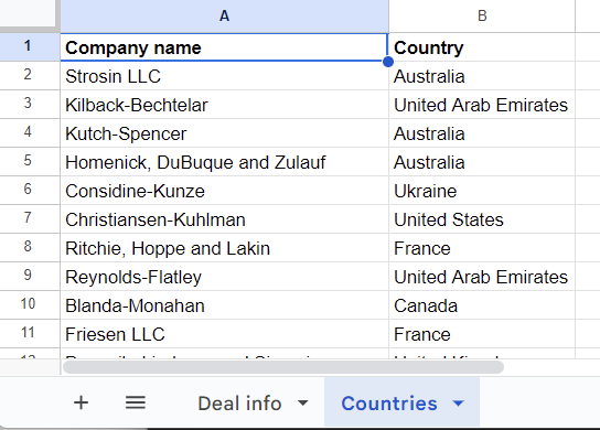
The second sheet, Deal info, contains a few columns with information about deals but the column Country is empty.
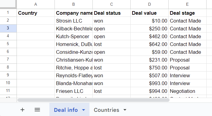
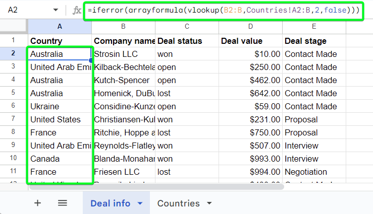
We need to populate this column with values from the Country column on the Countries sheet. This is what the VLOOKUP + ARRAYFORMULA can help us complete.
Once we insert the following formula in the A2 cell, we’ll get the Country column populated with the values related to the Company name values
=iferror(arrayformula(vlookup(B2:B,Countries!A2:B,2,false)))
No doubt, the ARRAYFORMULA-VLOOKUP combination, when used properly, is a tool that can save you tons of time and spare you a lot of busy work.
FILTER and ARRAYFORMULA in Google Sheets
Another popular and useful function that proves beneficial when you need to find information quickly is the FILTER function. It is used to conditionally filter the specified data range to get the required info. This Google Sheets function has already been explained in the FILTER How-To Guide, but let’s reconsider the application of FILTER with ARRAYFORMULA.
In the sales spreadsheet, let’s filter out duplicates – in our case, the identical sales numbers. Since there is no direct function in Google Sheets to cope with the task, the optimal workaround will be to use FILTER with UNIQUE, ARRAYFORMULA, and COUNTIF:
=filter(
   unique(C2:C),
   arrayformula(
      countif(C2:C,unique(C2:C))>1
   )
)
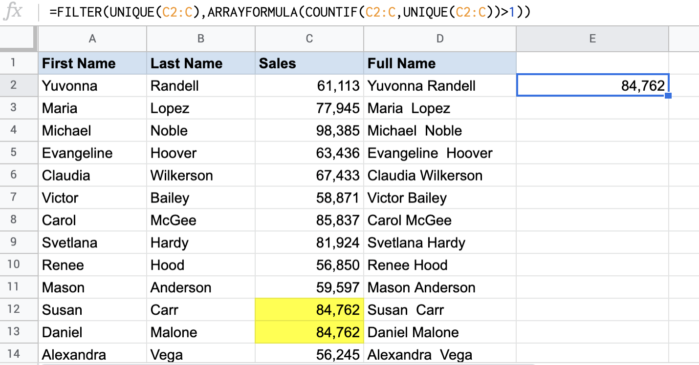
As you can see, the formula meets the challenges and returns one duplicate.
How to use ARRAYFORMULA to combine columns in Google Sheets
ARRAYFORMULA also helps you do manipulation with a text. You can actually combine a text with a text, a text with a number, and a text with a date in Google Sheets and apply ARRAYFORMULA to that combination.
For example, if we have a list of, let’s say, sales managers, and need to combine the first and last names. To get the name and the surname of the first sales manager, use the following formula:
=A2 &" "& B2
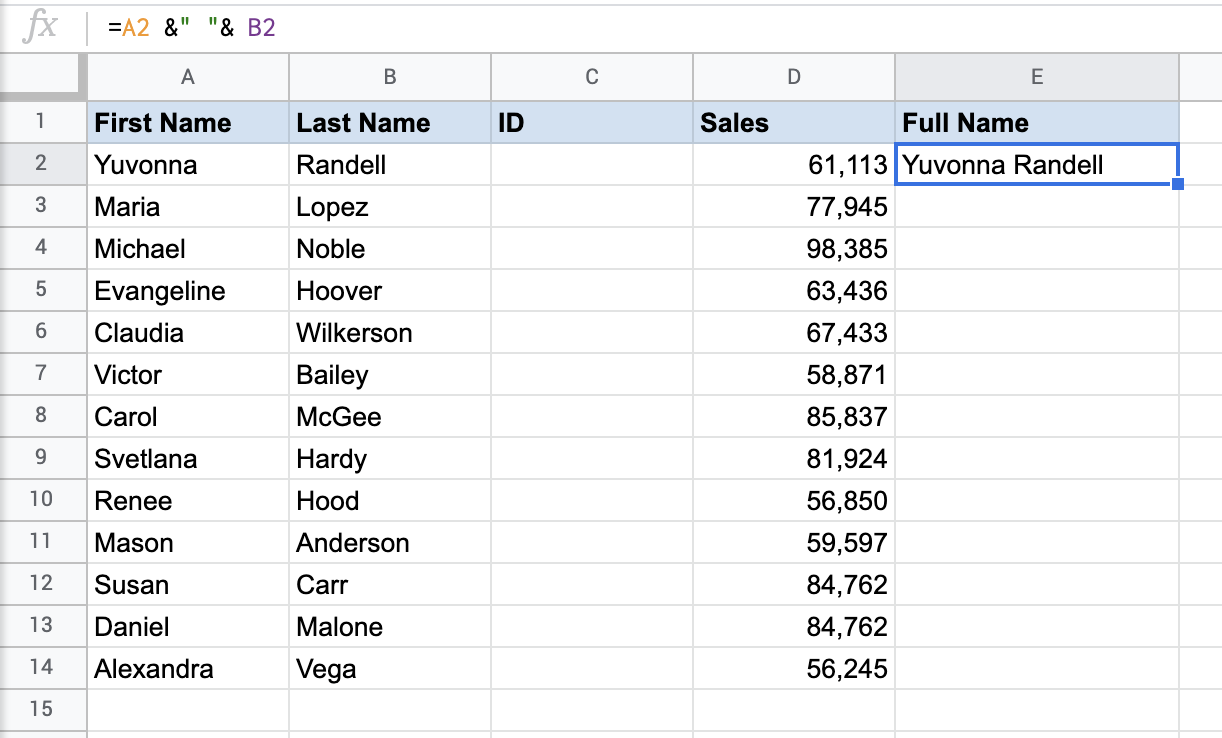
The full name appears in a single cell, E2. Read more about Merging Data in Google Sheets.
So, let’s use the ARRAYFORMULA function to have all the names and surnames coupled.
=arrayformula(A2:A14 &" "& B2:B14)
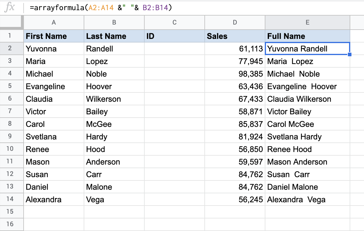
Applied only in E2, the formula automatically expanded to the other cells below.
Blank cells challenge in Google Sheets ARRAYFORMULA output
When you work with the ARRAYFORMULA function, you have to be careful with the array sizes. They should always be the same, for example, F2:F17&G2:G17. Otherwise, Google Sheets won’t carry out the calculation. As an option, not to sweat too much, you may use the infinite range, as we did with SUMIF.
=arrayformula(
   sumif(F2:F,H2:H,D2:D)
)
But, in this case, you may face another challenge – extra blank cells in your formula output. In my instance with ARRAYFORMULA+SUMIF in I2, if there is a limited range of H2:H4, all will work well.
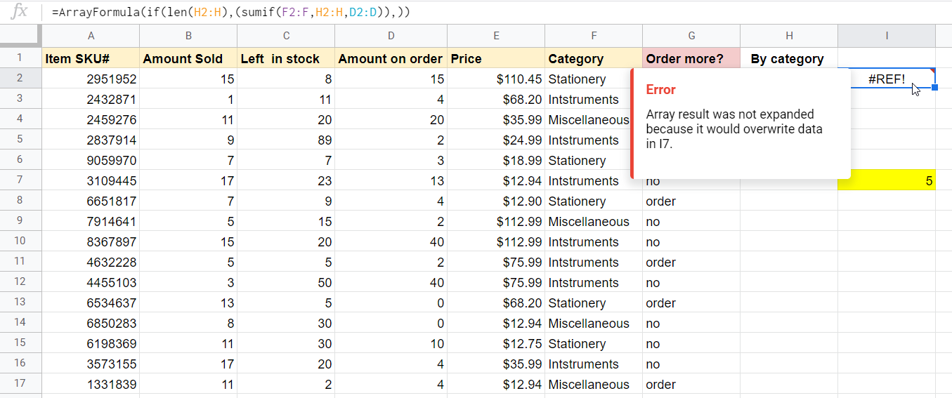
However, if you change it to H2:H, SUMIF will treat this range as the one containing the criteria and will sum the column accordingly.
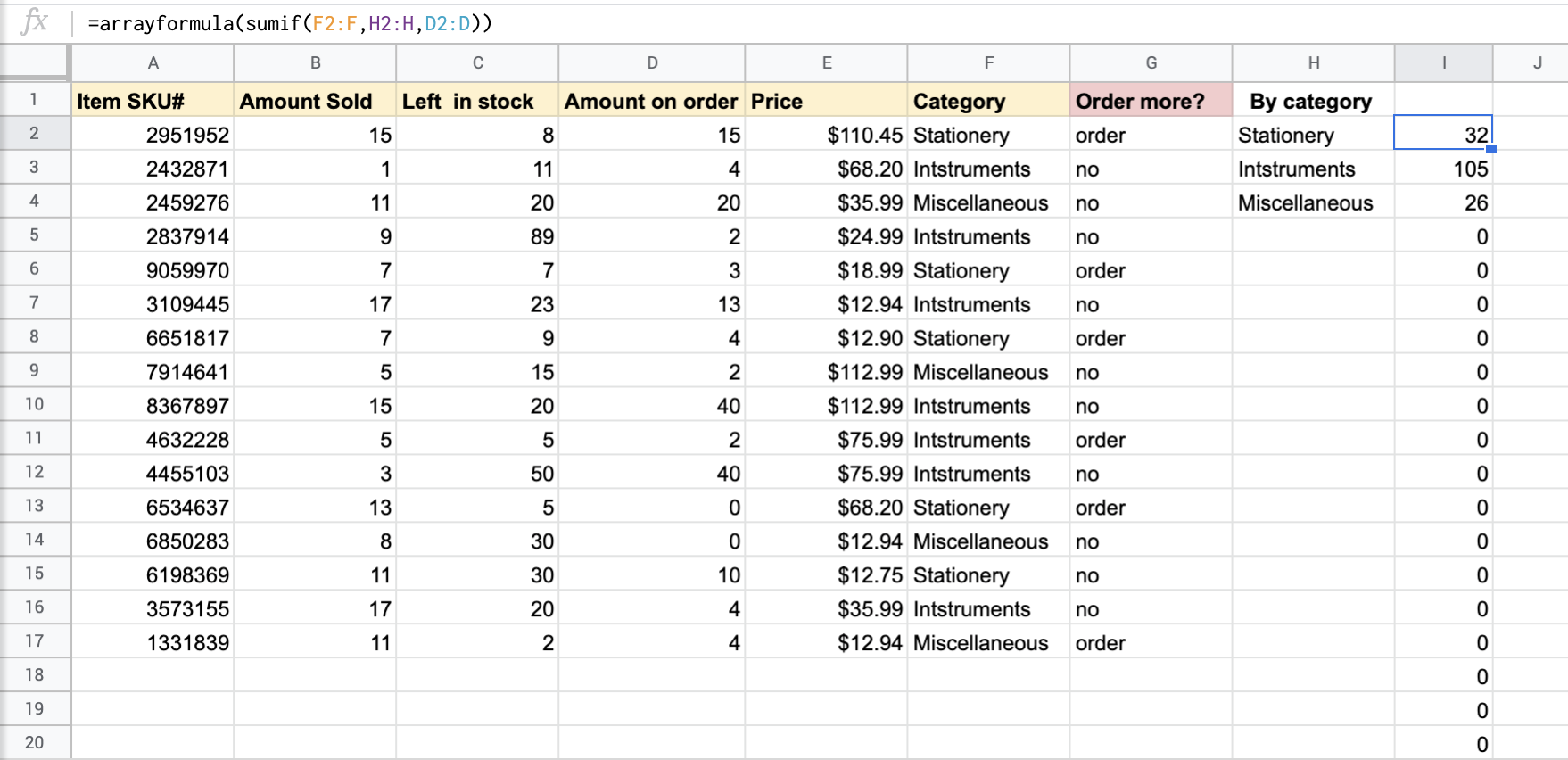
Well, it may spoil the looks, let alone litter up the whole spreadsheet, but, most importantly, when you enter any value in any of those cells, the formula will return a #REF! Error.
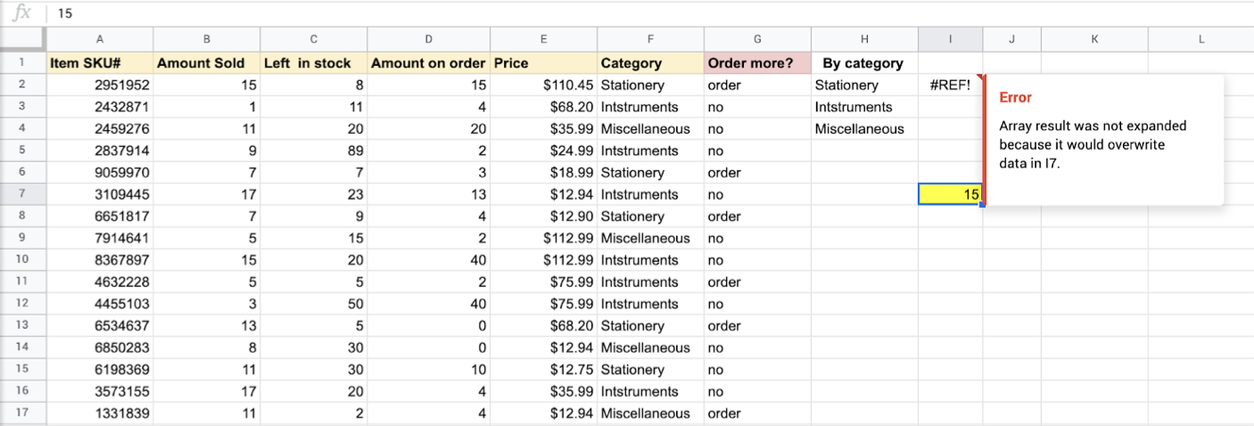
And this happens not only with SUMIF but with other formulas as well. So, let’s see how to remove them.
How to remove extra blank cells in ARRAYFORMULA Google Sheets output
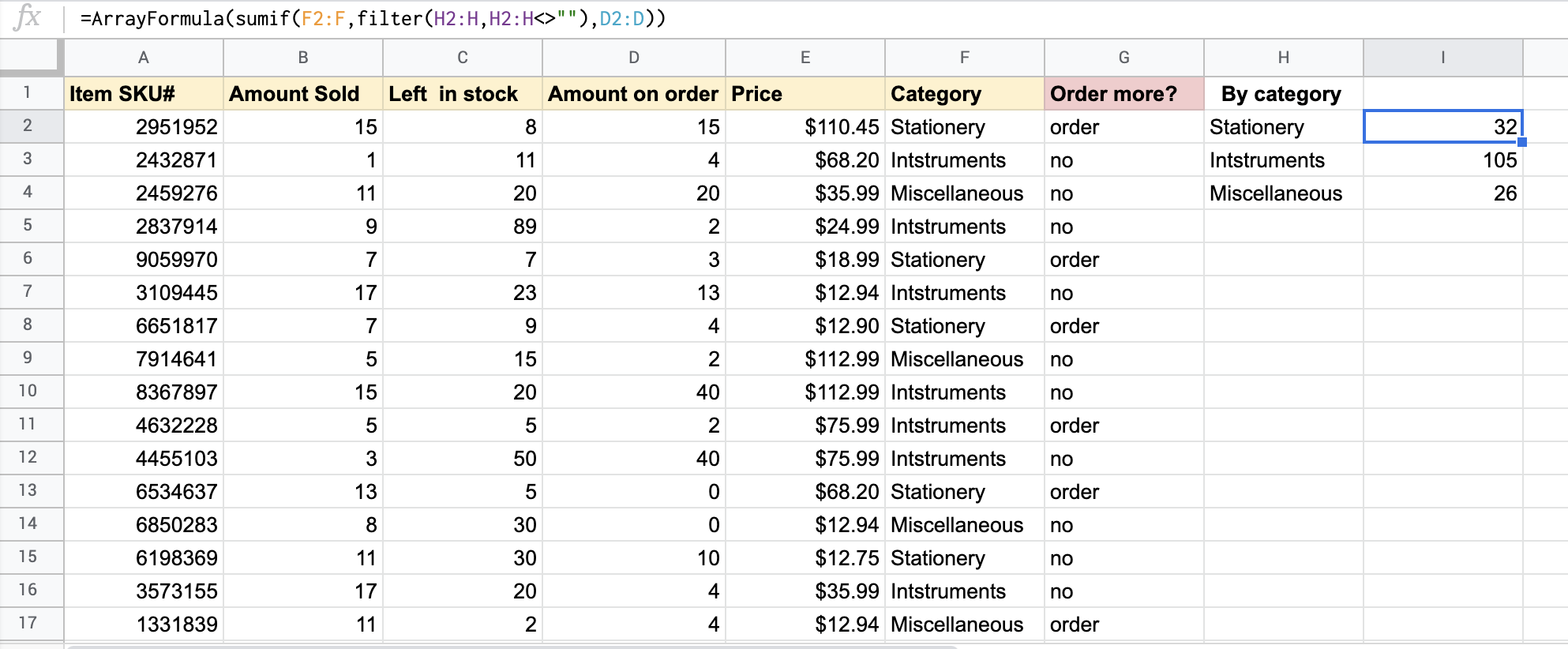
So, to remove extra blank cells returned by ARRAYFORMULA nested with SUMIF in Google Sheets, we can use the FILTER function to filter out blank cells in the criteria that cause the extra zeros and the blank cells correspondingly.
=ArrayFormula(
   sumif(F2:F,filter(H2:H,H2:H<>""),D2:D)
)
Or, alternatively, you can use IF+LEN and it will do the same job.
=ArrayFormula(
   if(len(H2:H),(sumif(F2:F,H2:H,D2:D)),)
)
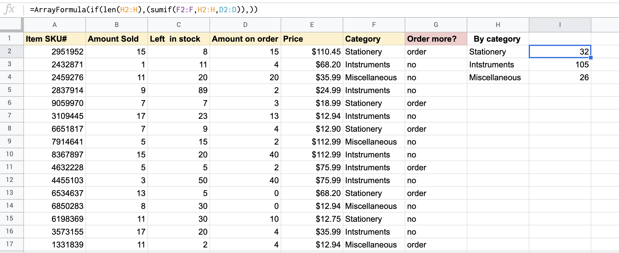
But, unlike the option with FILTER, IF+LEN won’t help to avoid the issue with #REF! Error and will also return it if you enter any value in blank cells, so be careful!
That’s the curtain?
Hardly. The Google Sheet ARRAYFORMULA function is a really multi-purpose tool and can be used with many other combinations and applications not covered here. If you have any in mind and want to discuss them, comment below and we’ll elaborate.
As for now, good luck with your data, and as Ben Collins, Google Sheets developer and data analytics instructor, wrote in his blog, “Hip, Hip Array!”