BigQuery Tutorial – How to Use BigQuery for Your Projects

What should a perfect BigQuery Tutorial consist of? It should probably answer three questions: what, why, and how? We have dared to write such a perfect piece and go beyond. Our goal is to look at BigQuery from the business perspective: what business benefits this cloud data warehouse has compared to its competitors. Read on and tell us whether we succeeded and our tutorial hit the target. 🙂

What is Google BigQuery?

In our opinion, there can be a few answers to this question: 

BigQuery is a database 

In the widest sense, BigQuery is a database. As you know, databases are collections of related data, and BigQuery allows you to store terabytes of records.  

BigQuery is a cloud data warehouse

Data warehouse is BigQuery’s official title. Data warehouses are systems that allow you not only to collect structured data from multiple sources but also analyze it. So, you can call it an analytics database for querying and getting insights from your data.

BigQuery is a columnar database

This title rests on BigQuery’s columnar storage system that supports semi-structured data — nested and repeated columns. This is mostly a technical definition, which we have introduced to broaden your horizons.

BigQuery is a spreadsheet database ?

This is a down-to-earth definition of BigQuery if the ones above are not enough. BigQuery combines the features of both spreadsheet software, such as Google Sheets, and a database management system, such as MySQL. 

Why you should use BigQuery

The main reason to opt for BigQuery is analytical querying. BigQuery allows you to run complex analytical queries on large sets of data. Queries are requests for data that can include calculation, modification, merging, and other manipulations with data. 

Let’s say, in Google Sheets, you can also query data sets using the QUERY function. This may work for different kinds of reports and charts based on small to medium data sets. However, any spreadsheet app (even Excel) won’t be able to handle complex queries of large data sets that include millions of rows in a table.

BigQuery is aimed at making analytical queries beyond simple CRUD operations and can boast a really good throughput. However, in our BigQuery tutorial, we do not claim it to be the best database solution, and definitely not a replacement for a relational database. 

BigQuery setup guide 

Another reason why you may consider BigQuery is that it’s a cloud service. You don’t have to install any software. Google handles the infrastructure and you just need to set up BigQuery, which is quite easy.  

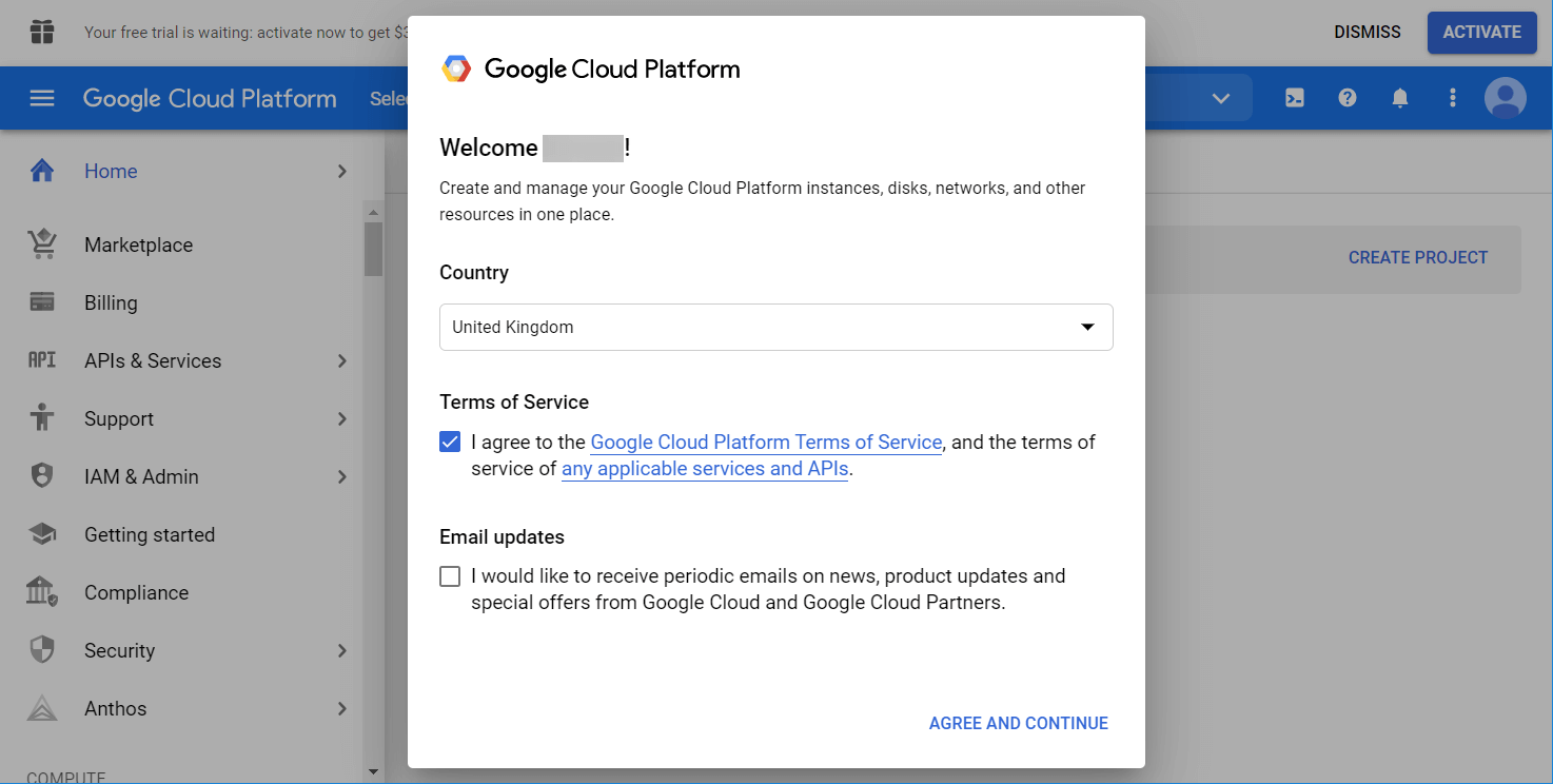
Your journey will start with the Google Cloud Platform. If it’s your first visit, you’ll need to select your country and agree to the Terms of Service.

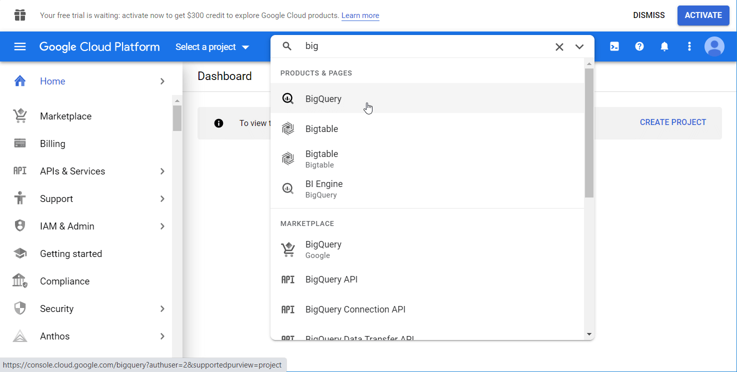
After that, go to BigQuery – you can use either the search bar or find it manually in the left menu.

Create a BigQuery project

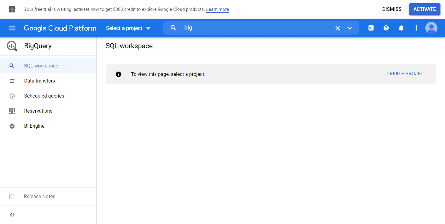
Here is what BigQuery looks like on your first visit.

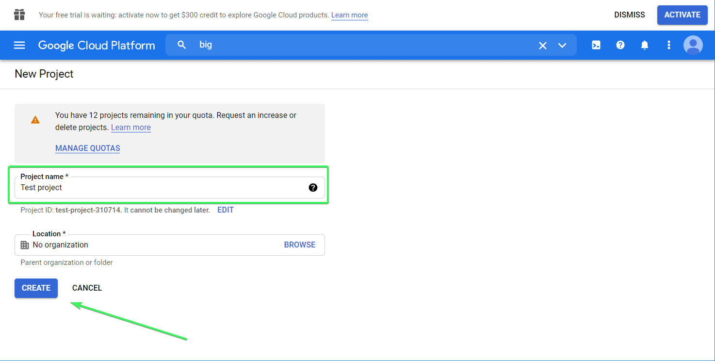
Click the Create Project button to spin the prop. Name your project, choose the organization if needed, and click Create. 

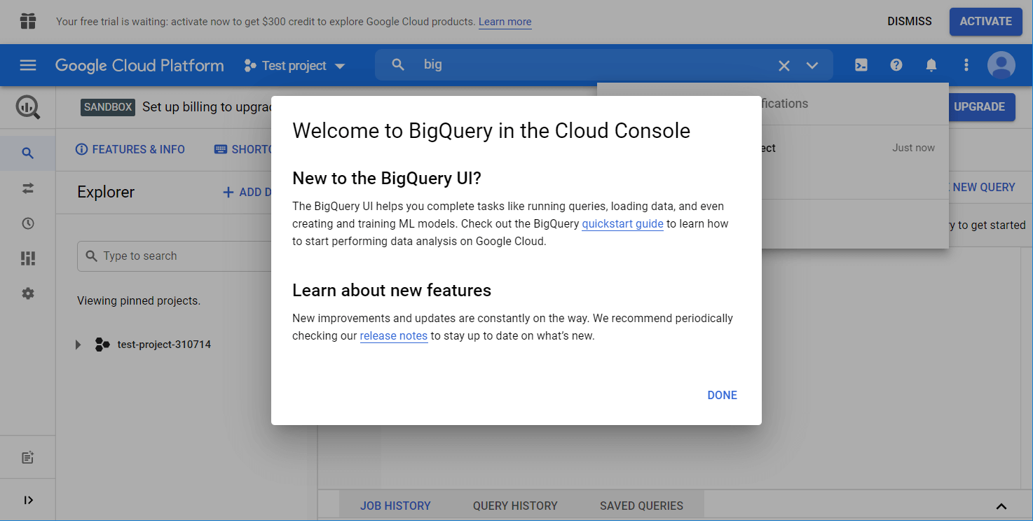
Now you’re officially welcomed to BigQuery. 

What is a BigQuery sandbox?

Two messages on the top of the BigQuery console have likely drawn your attention.

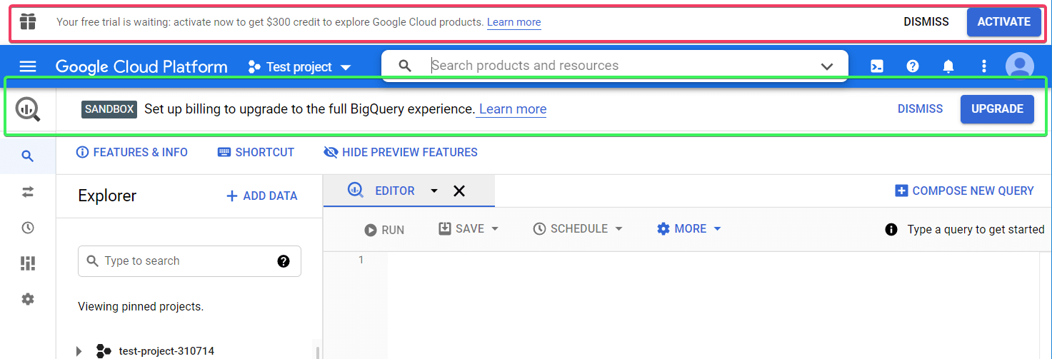
SANDBOX means that you’re using a sandbox account, which does not require you to enter payment information. This free tier option grants you 10 GB of active storage and 1 TB of processed query data per month. Using this account, your tables will expire in 60 days. Click Learn more to discover other limits.

The second banner offers you to activate a free trial. The difference from the sandbox account is that if you activate the trial, you’ll need to enter your billing details. If you do, you’ll get $300 of cloud credits free.

For our Google BigQuery tutorial, we’ll be using the sandbox option. So, feel free to click Dismiss for both options.

How to use Google BigQuery

Create a data set in BigQuery

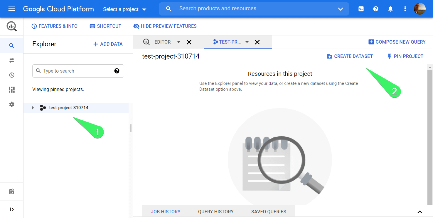
Let’s add some data into BigQuery to check out how it works. Click the project you want, and then Create Dataset. 

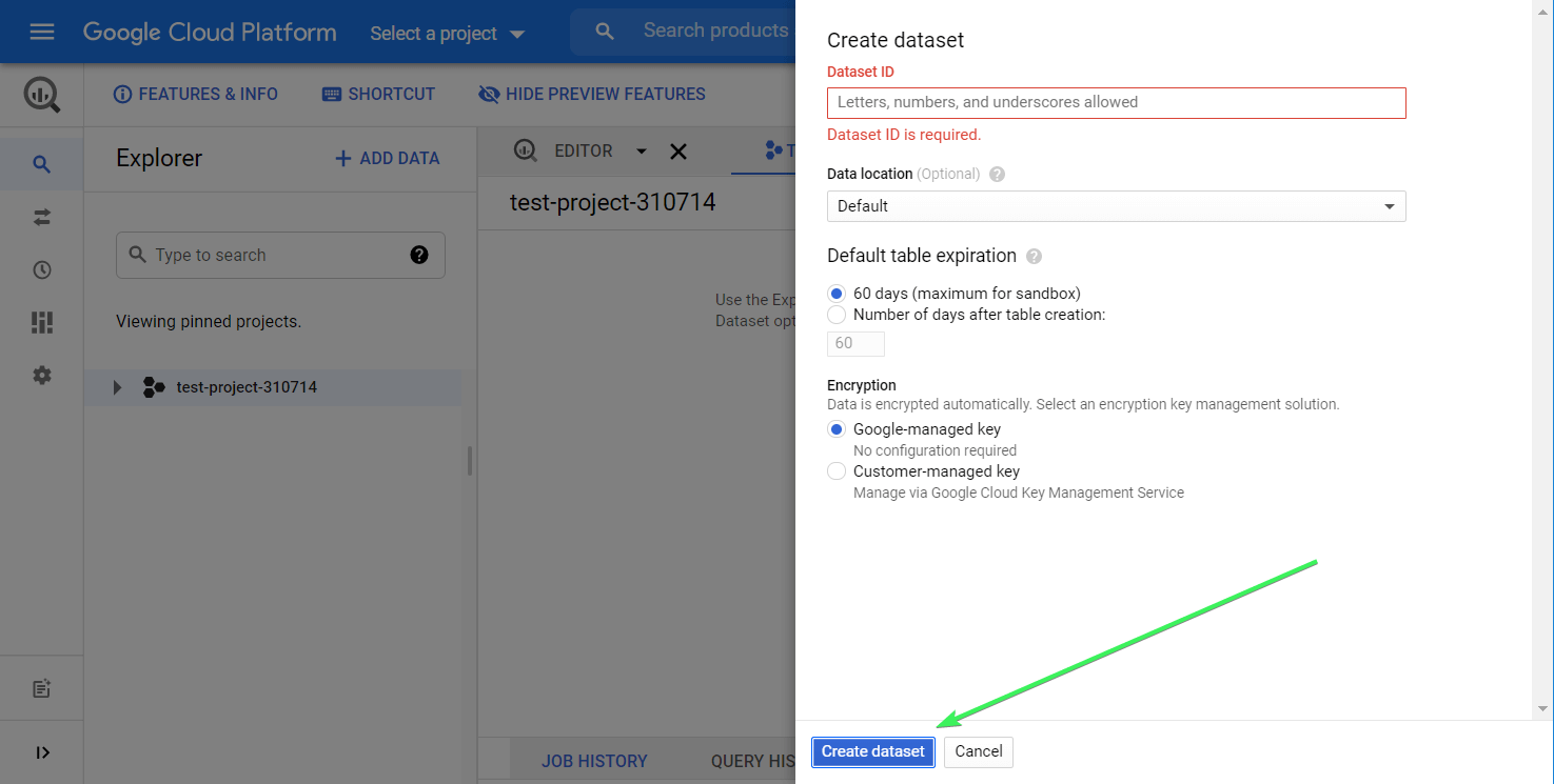
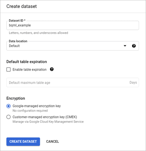
Assign a Dataset ID – you can enter letters and numbers. If needed, you can select the Data location as well as a table expiration (up to 60 days) and encryption. After that, click Create dataset.

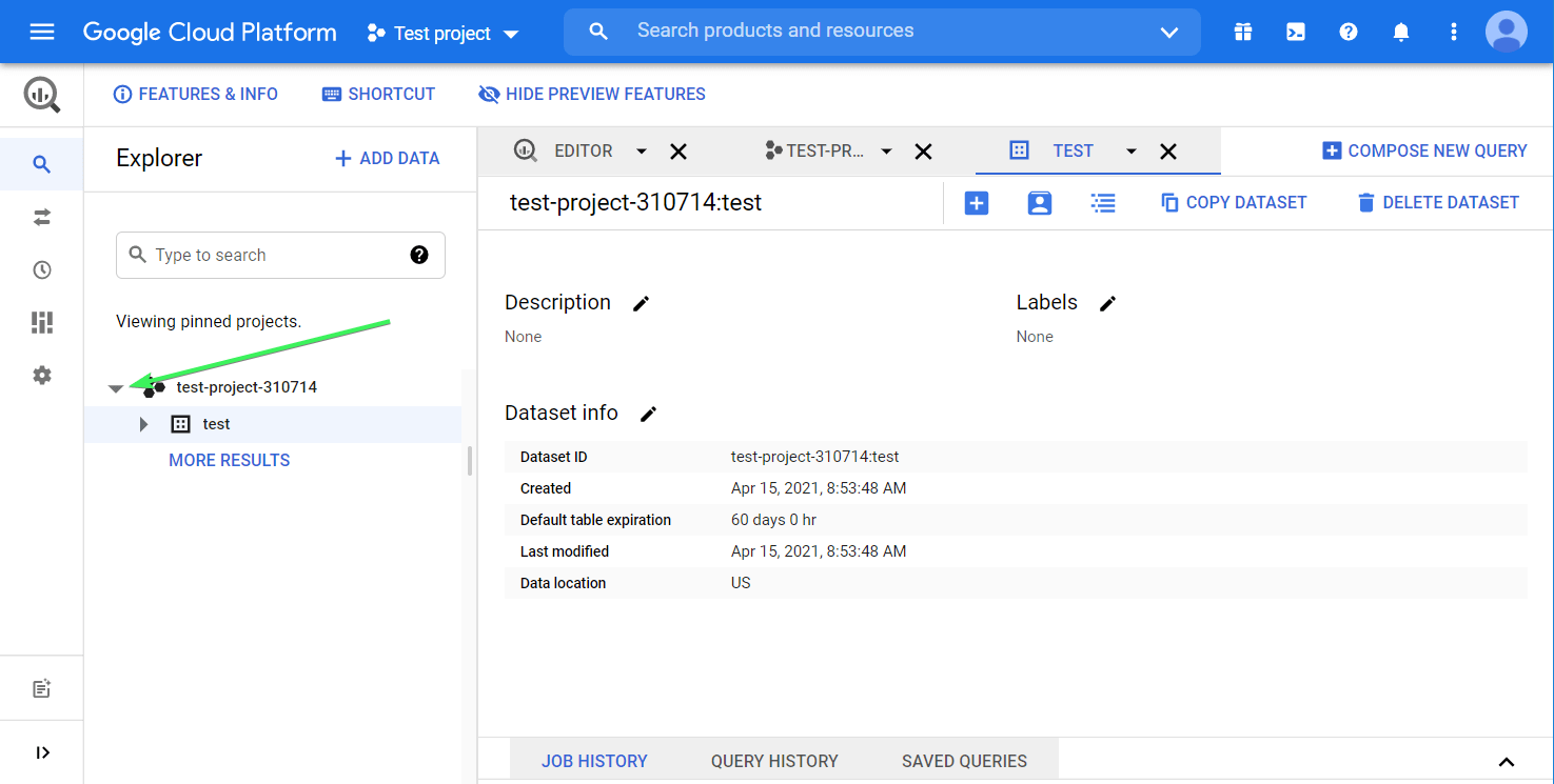
A new dataset is now created. You can find it by clicking the Expand node button next to your project name:

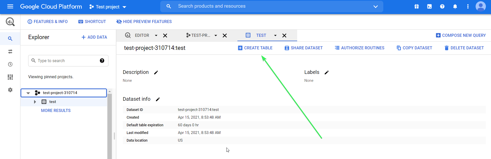
The next step is to create a table in the dataset. Here is the button to click:

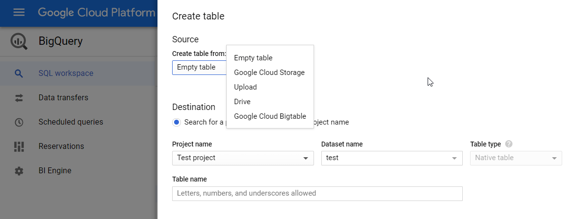
You have a few options here:

• Create an empty table and fill it manually
• Upload a table from your device in one of the supported formats (explained in the next section)
• Import a table from Google Cloud Storage or Google Drive (this option allows you to import Google Sheets)
• Import a table from Google Cloud Bigtable through the CLI

File formats you can import into BigQuery

You can easily load your tabular data into BigQuery in the following formats:

• CSV
• JSONL (JSON lines)
• Avro
• Parquet
• ORC
• Google Sheets (for Google Drive only)
• Cloud Datastore Backup (for Google Cloud Storage only)

Note: BigQuery does not support import of Excel files. To do this, you’ll need to either convert your Excel file to CSV, or convert Excel to Google Sheets and then load it to BigQuery. The best option, however, is to use Coupler.io that allows to export data from different sources to BigQuery, including Excel. 

Automate import to BigQuery from your data sources with Coupler.io

Let’s say you have the data set in Google Sheets or another app you need to load to BigQuery every day. You can do this manually or automate the data import by using Coupler.io. 

1. Collect data

To get started, select your data source and click Proceed in the form below. You’ll be prompted to sign up for free:

Connect to your data source and select the data to export. This could be spreadsheets in Google Sheets, reports from Google Ads, metrics from Google Analytics, and so on. 

2. Organize and transform data

Check the data you are going to export. In this step, you can:

• Rename, rearrange, hide, or add extra columns.
• Apply filters and sort data.
• Create new columns with custom formulas.
• Union data from multiple sources.

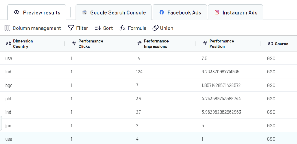
If your data looks correct, click Proceed.

3. Set up the destination

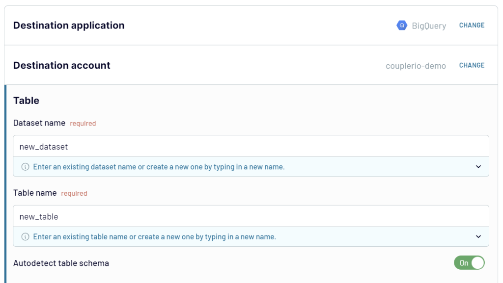
Connect your BigQuery account. For this, create a service account with two roles: BigQuery Data Editor and BigQuery Job User. Next, download and add your .json key file. Here is a detailed instruction. 

Then, enter the names of the BigQuery dataset and the table where the data from Google Sheets will be loaded.

Toggle on the Automatic data refresh and schedule your data exports. You can specify an update interval from every month to even every 15 minutes, making your report live.

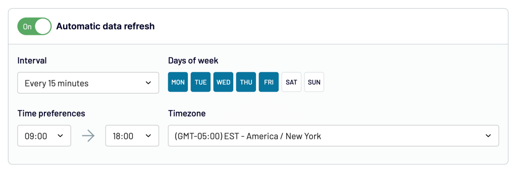
Finally, click Run Importer.

Upload CSV data to BigQuery

Once you click the Create table button, you need to complete the following steps:

1. Choose source – Upload
2. Select file – click Browse and choose the CSV file from your device
3. File format – choose CSV, but usually, the system auto-detects the file format
4. Table name – enter the table name
5. Check the Auto detect checkbox 
6. Click Create table

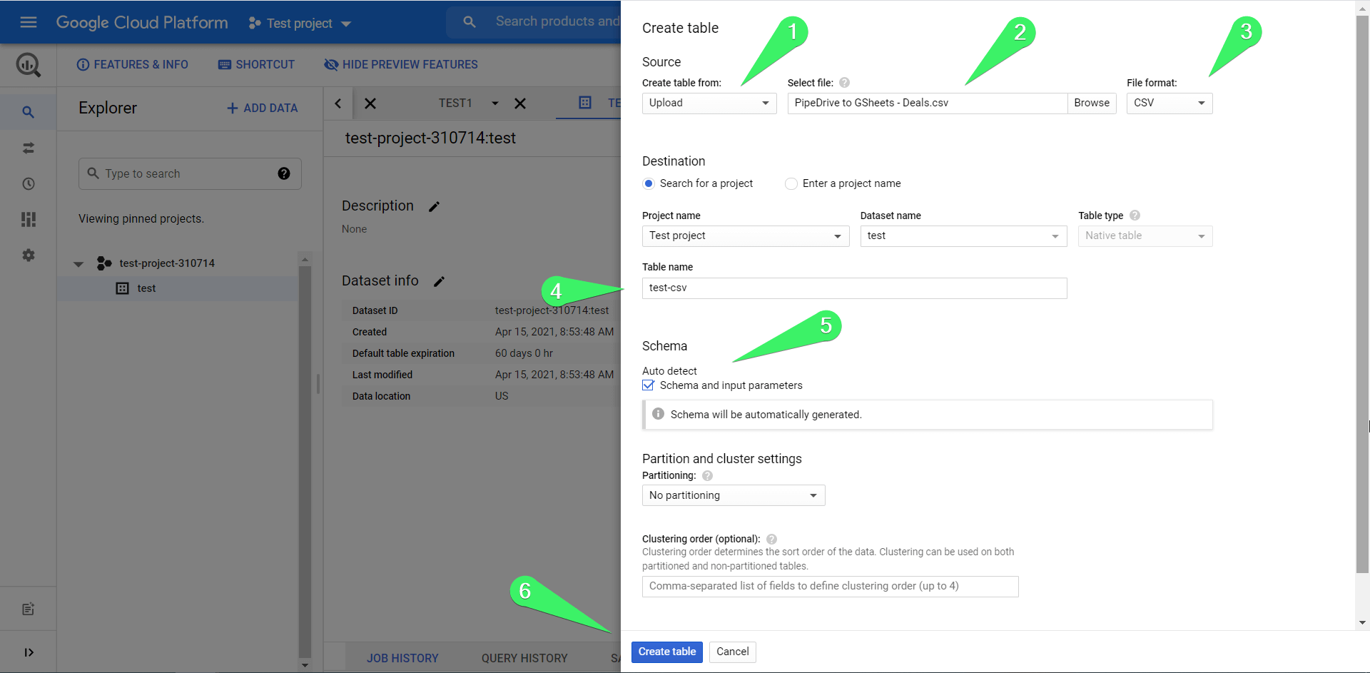
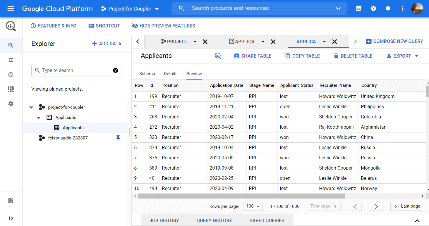
This is what the basic flow looks like. Additionally, you can define partition settings (to divide your table into smaller segments), cluster settings (to organize data based on the contents of specified columns), as well as configure the Advanced options. This is what your table uploaded to BigQuery looks like:

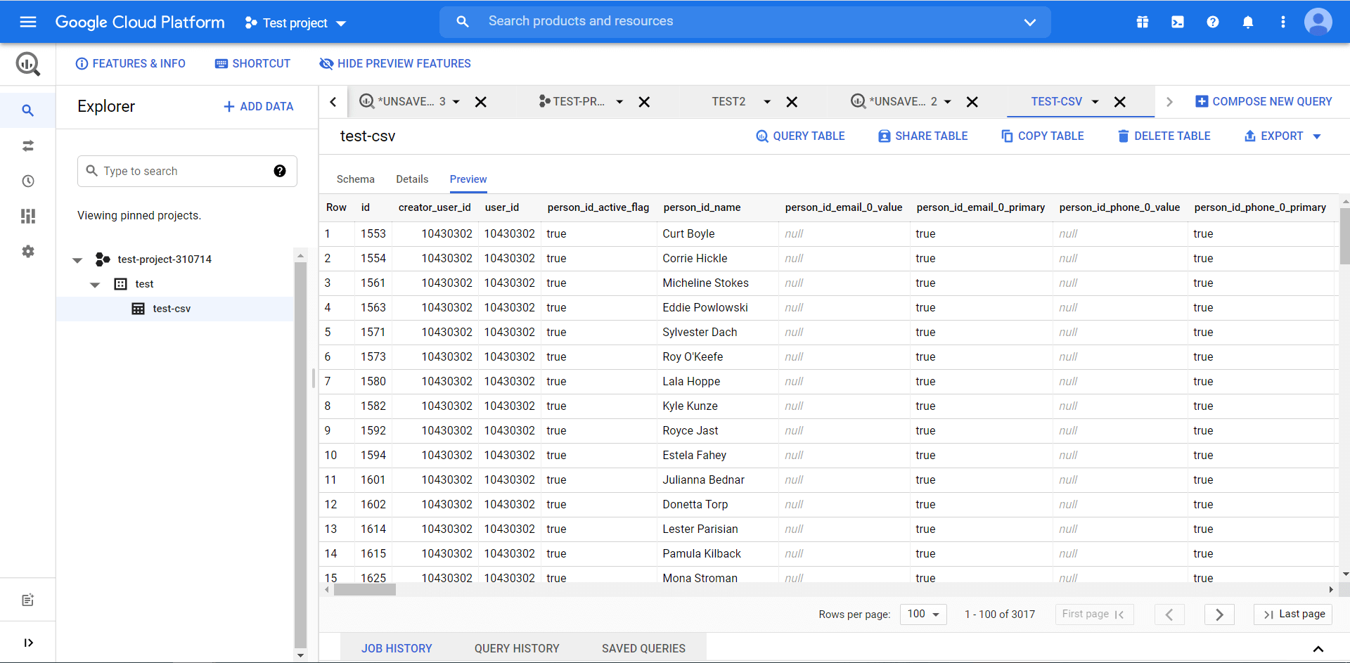
Note: The table preview feature shows previews for tables stored inside BigQuery. For example, when you upload CSV, it is saved in BigQuery – you’ll see the preview. However, when you pull data from Google Sheets, it is a real-time connection since BigQuery scans Google Sheets every time you query it. In this case, you won’t have the preview available.

Import data from Google Sheets to BigQuery manually

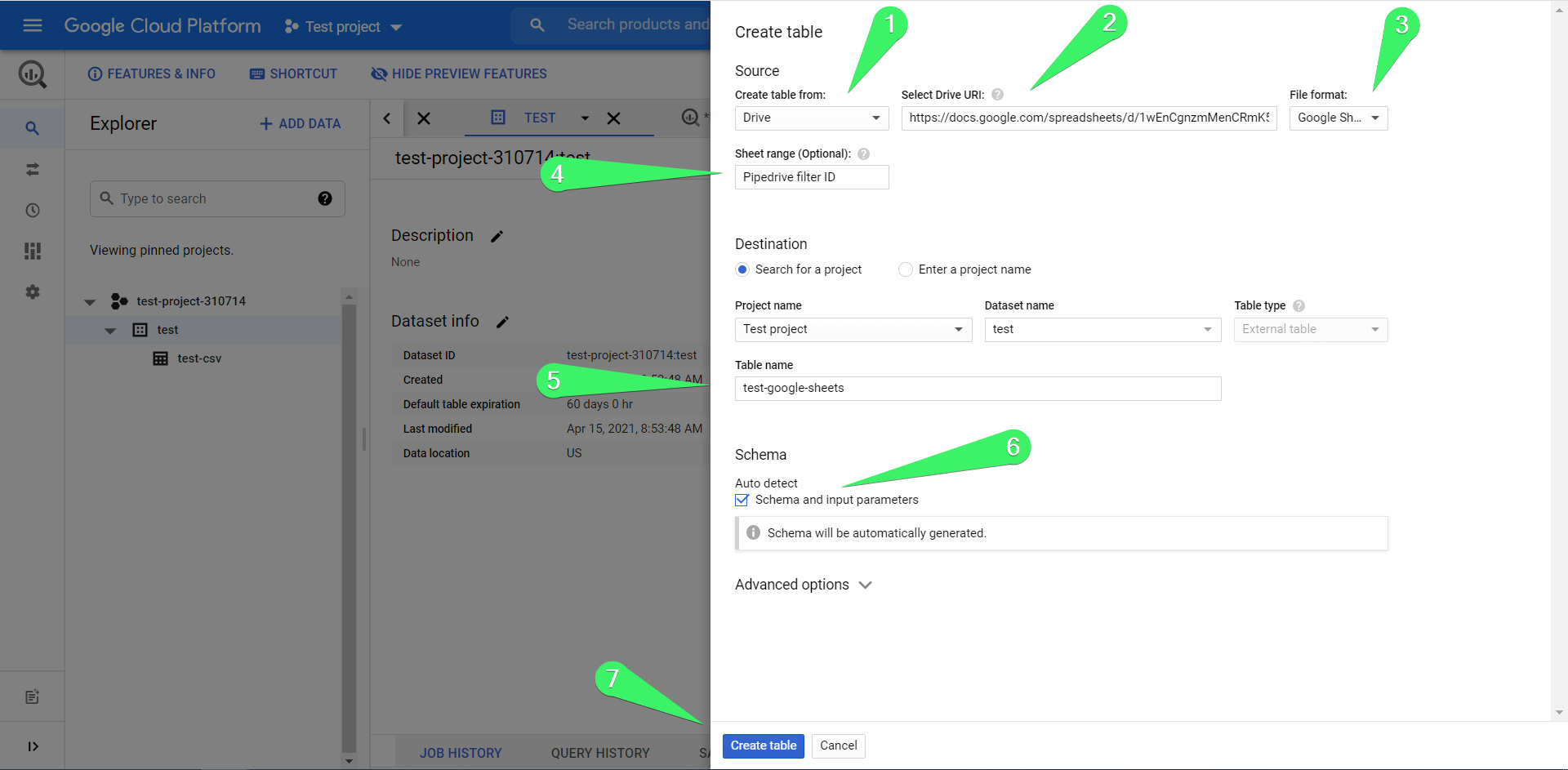
Most of you would probably like to learn more about importing tables from Google Sheets to BigQuery. The workflow is very similar but with a few modifications. Click the Create table button and:

• Choose source – Drive
• Select Drive URI – insert the URL of your Google Sheets spreadsheet 
• File format – choose Google Sheets
• Sheet range – specify the sheet and data range to import. If you leave this field blank, BigQuery will retrieve the data from the first sheet of your spreadsheet.
• Table name – enter the table name
• Mark the Auto detect checkbox 
• Click Create table

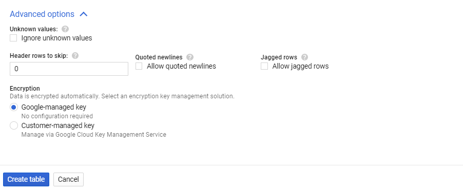
You may be interested in setting up Advanced options since they let you:

• Skip rows with the column values that do not match the schema.
• Skip a specific number of rows from the top.
• Enable including newlines contained in quoted data sections.
• Enable accepting rows that are missing trailing optional columns.
• Select an encryption key management solution.

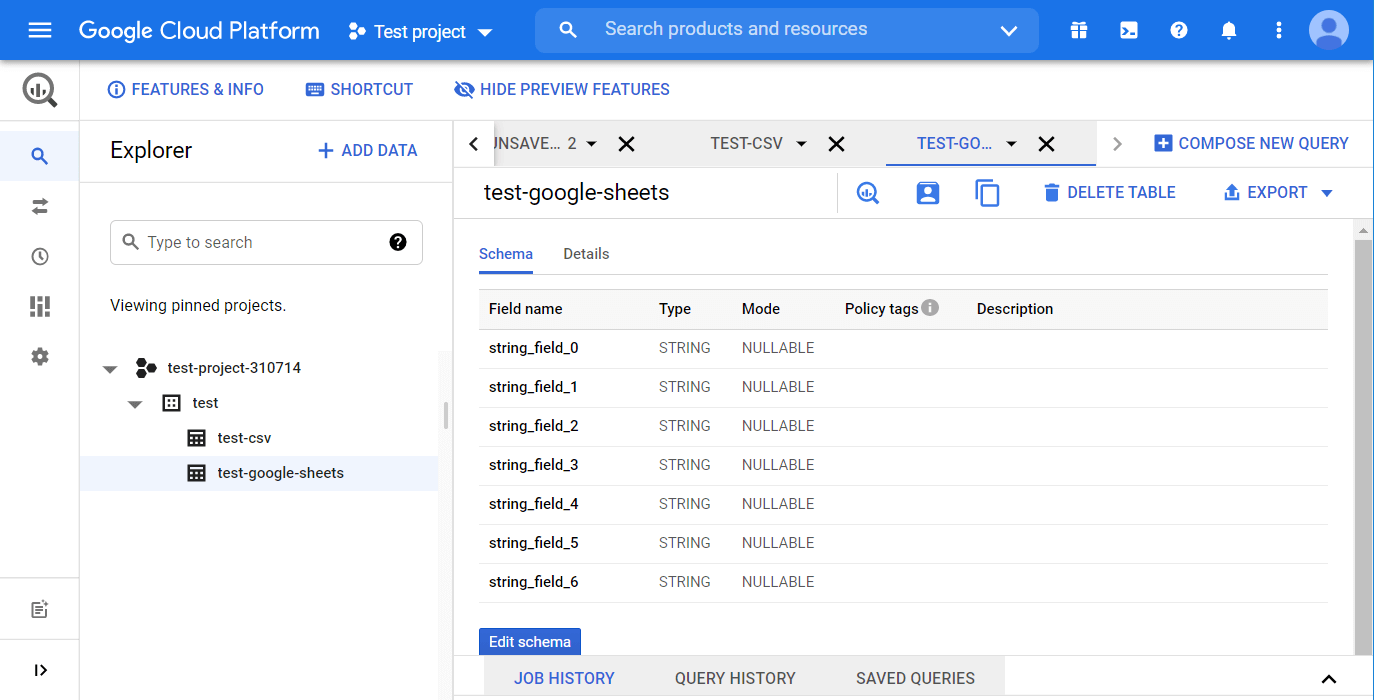
Once you click Create table, the specified sheet from your spreadsheet will be imported into BigQuery. Here are the details (table preview is not available for importing Google Sheets):

Query tables in BigQuery

The real power of BigQuery lies in querying. You can query the tables in your database using the standard SQL dialect. The non-standard or legacy SQL dialect is also supported, but BigQuery recommends using the standard SQL dialect.

Check out our Google BigQuery SQL Tutorial to delve into this.

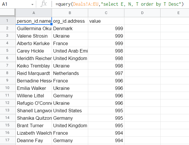
If you know what the Google Sheets QUERY function looks like, then you should understand how queries work. For example, here is a QUERY formula example:

=query(Deals!A:EU,"select E, N, T order by T Desc")

"select E, N, T order by T Desc" – this is the query to retrieve three columns of the entire data set and order the results in descending order.

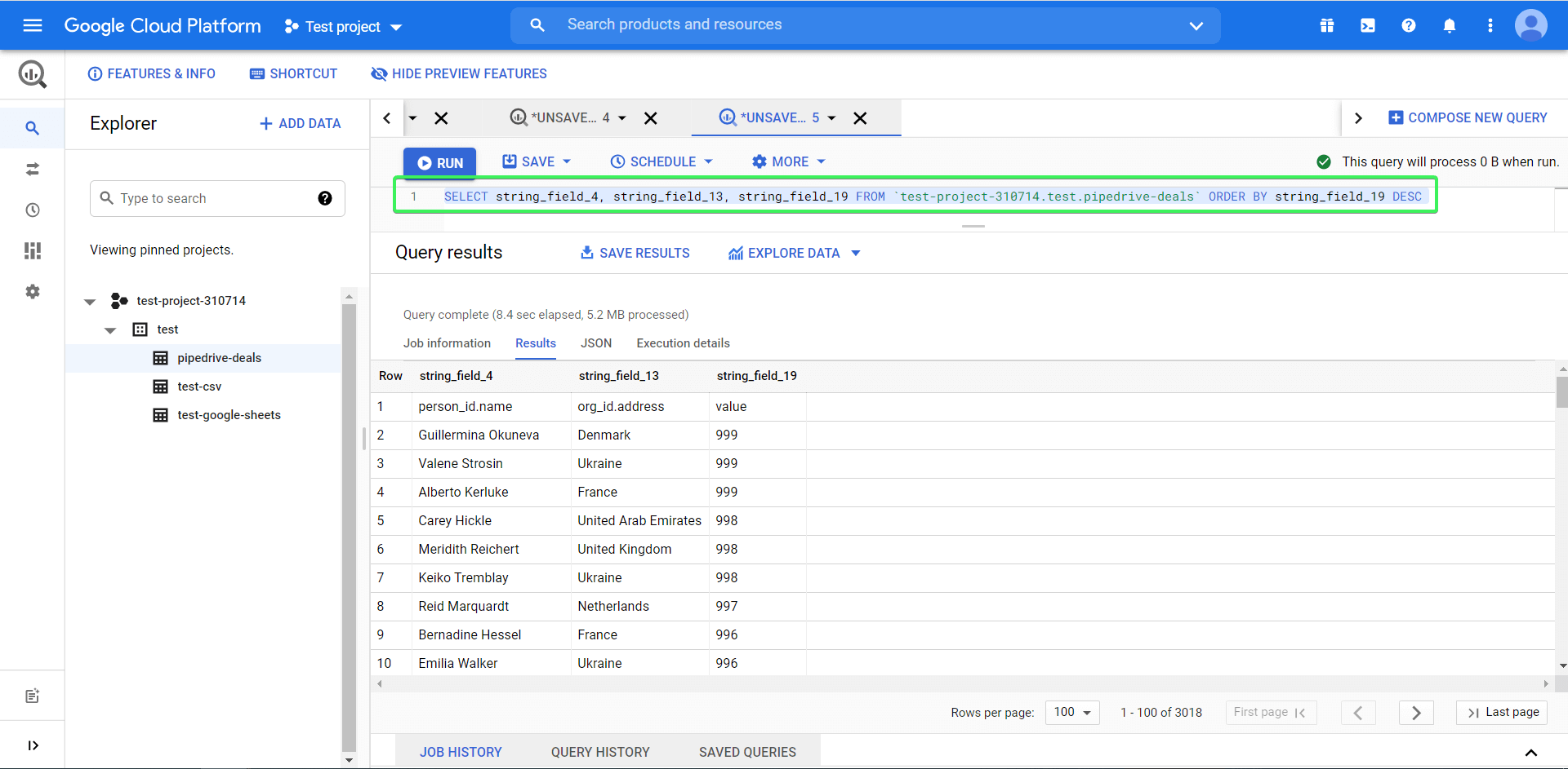
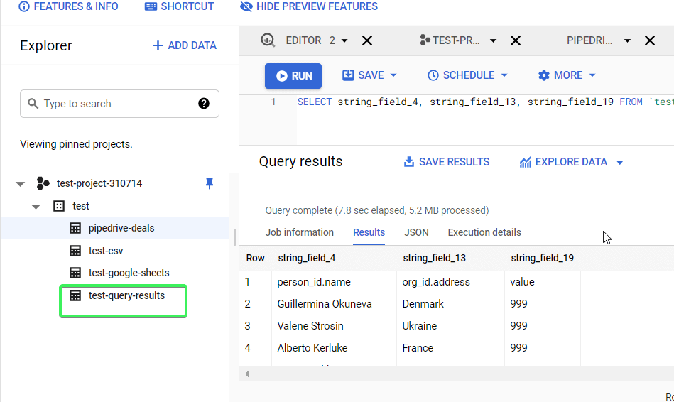
In BigQuery, the same query on the dataset imported from Pipedrive to BigQuery will look like this:

SELECT 
       string_field_4, 
       string_field_13, 
       string_field_19 
FROM `test-project-310714.test.pipedrive-deals` 
ORDER BY string_field_19 DESC

 Now we’ll explain how it works.

How to query data in BigQuery + syntax example

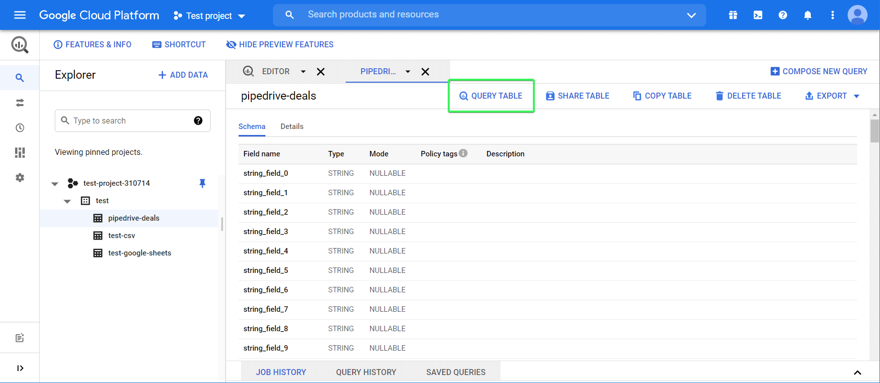
Click the Query table button to start querying.

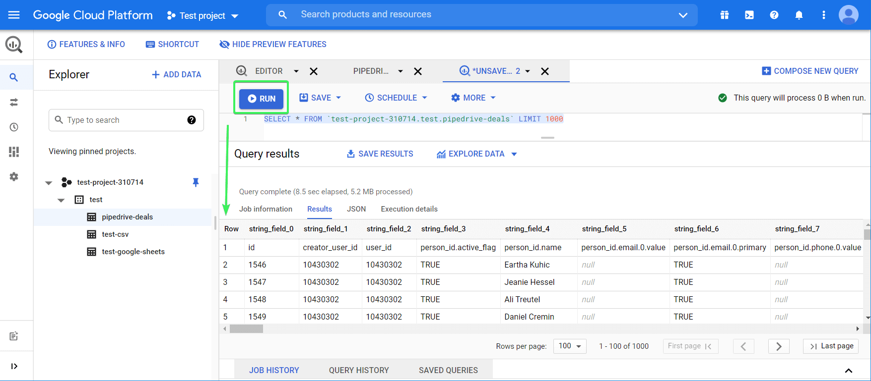
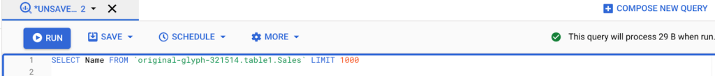
You’ll see the query boilerplate, like this:

SELECT FROM `test-project-310714.test.pipedrive-deals` LIMIT 1000

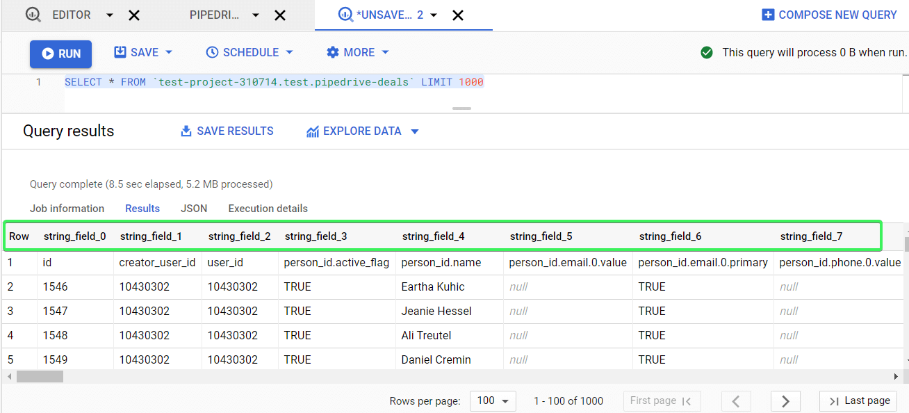
This is the basic example you can use to start your introduction to querying. Add * after the SELECT method, so that the query looks like this:

SELECT * FROM `test-project-310714.test.pipedrive-deals` LIMIT 1000

This query will return all available columns from the specified table, but no more than 1,000 rows. Click Run, and there you go!

Now, let’s query specific fields (columns) and order them. So, instead of using *, we need to specify the field names we need. You can find the field names in the Schema tab, or from your last query.

Let’s replace the LIMIT method from the default query with ORDER BY – this will let you sort data by a specified column. To sort data in descending order, add DESC to the end of the query. Here is what it looks like:

SELECT 
       string_field_4, 
       string_field_13, 
       string_field_19 
FROM `test-project-310714.test.pipedrive-deals` 
ORDER BY string_field_19 DESC

Here is our Google BigQuery SQL tutorial. You can also check out this SQL Video Tutorial for Beginners, made by Railsware. 

Query settings

If you click More and select Query Settings, you’ll be able to configure the destination for your query results and other settings.

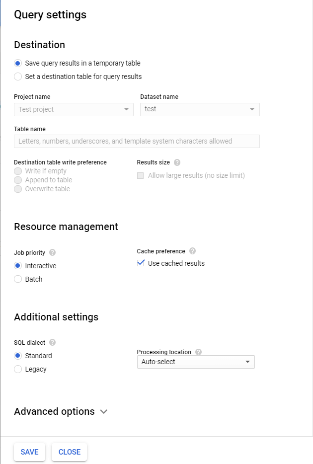
Here you can also set up to run queries in batches. Batch queries are queued and started as soon as idle resources are available in the BigQuery shared resource pool.

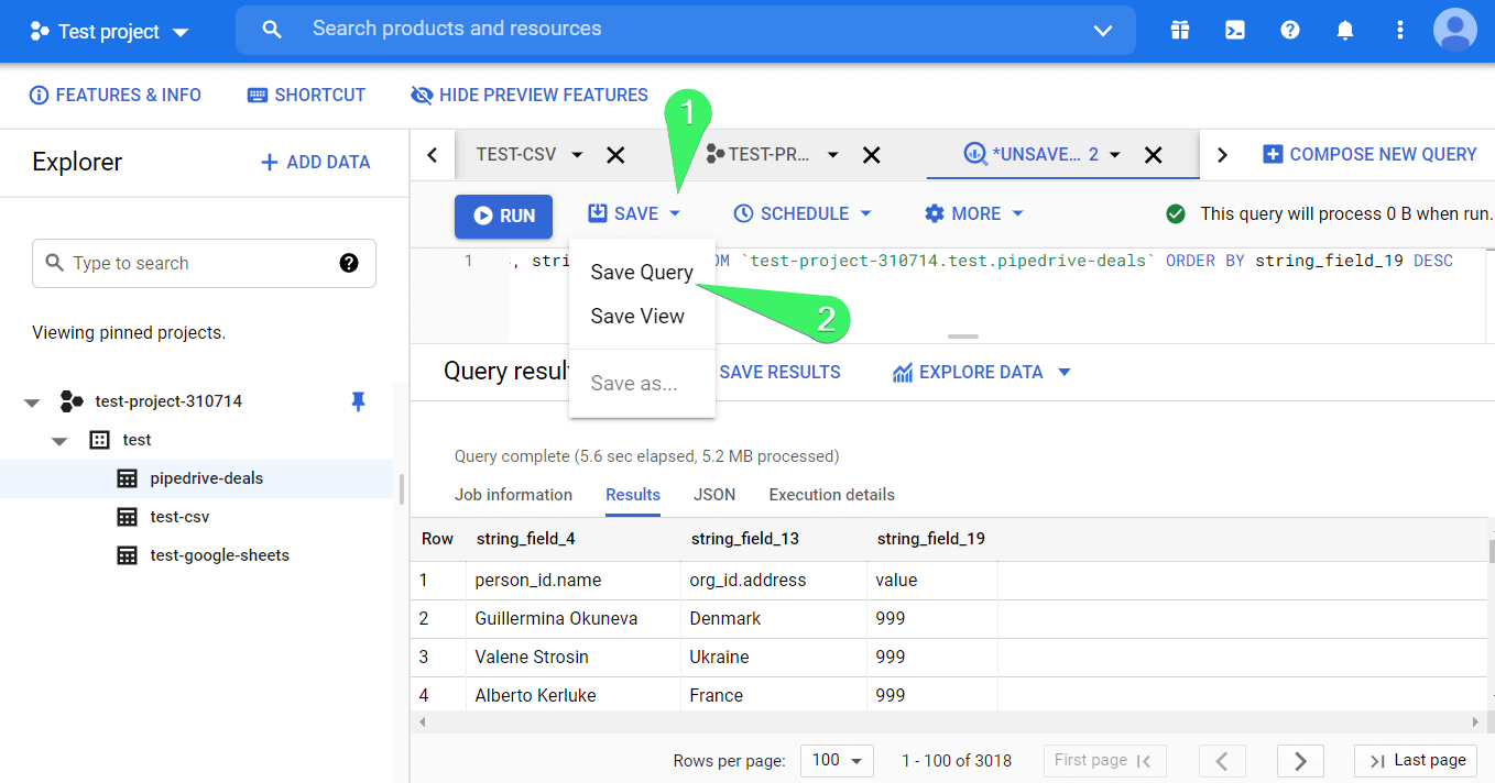
How to save queries in BigQuery

You can save your queries for later use. To do this, click Save => Save Query.

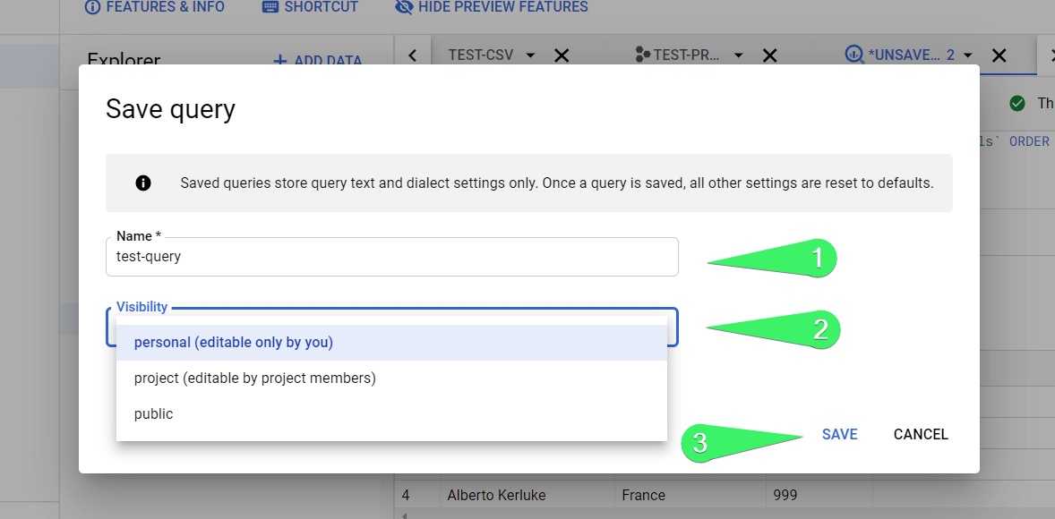
In the next window, name your query and choose its visibility:

• personal – only you will be able to edit the query
• project – only project members will be able to edit the query
• public – the query will be available publicly for edit

Click Save.

You can find your saved queries in the respective popup tab.

How to schedule queries in BigQuery

Next to the Save button, there is a Schedule button, which allows you to enable scheduled queries. Your first thought: “Why would I run queries on a schedule?” Well, there are at least two reasons to do this:

• Queries can be huge and take a lot of time to run, so it is better to prepare data in advance.
• Google charges money for data queries, so if it is OK for you to have data updated daily, it is better to do that and use the already prepared views to query them ad-hoc.

Note: Query scheduling is only available for projects with billing enabled. It won’t work for SANDBOX account projects.

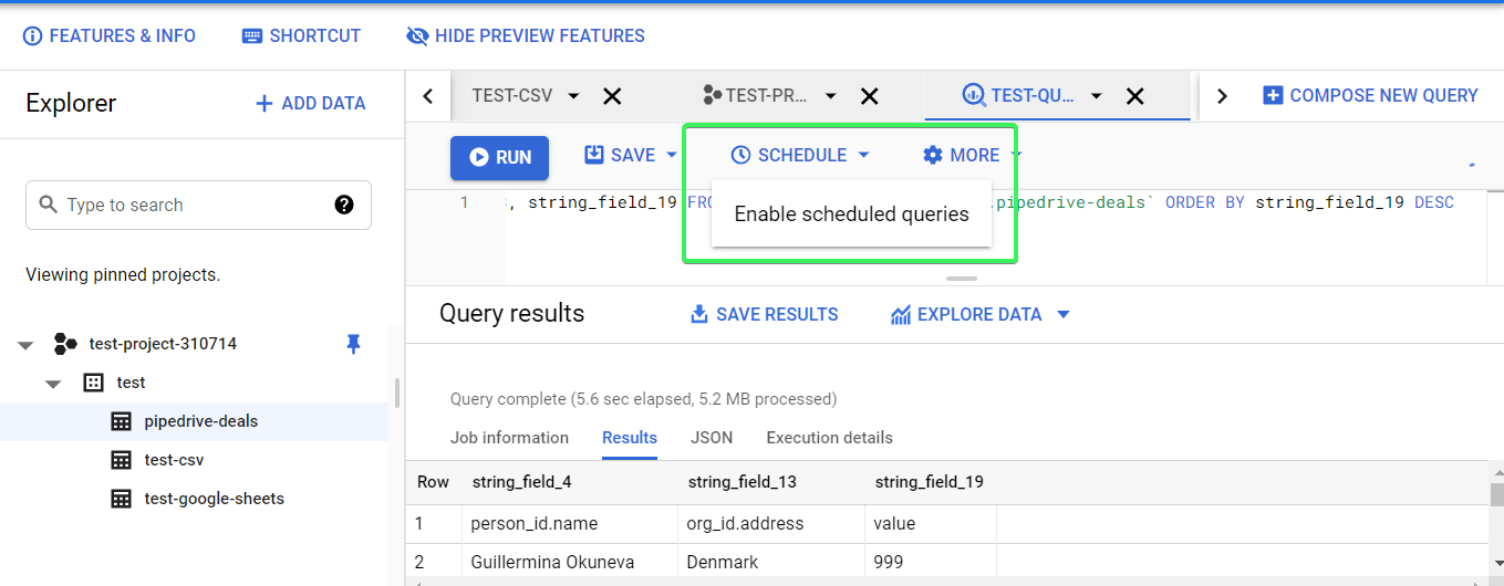
Once you click the Schedule button, you’ll get a notification that you need to first enable the BigQuery Data Transfer API. 

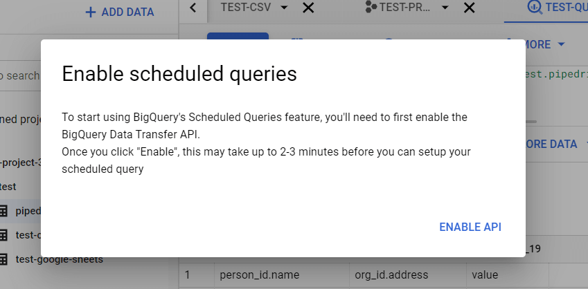
Click Enable API and wait a short time. After that, you’ll be able to create scheduled queries when you click the Schedule button.

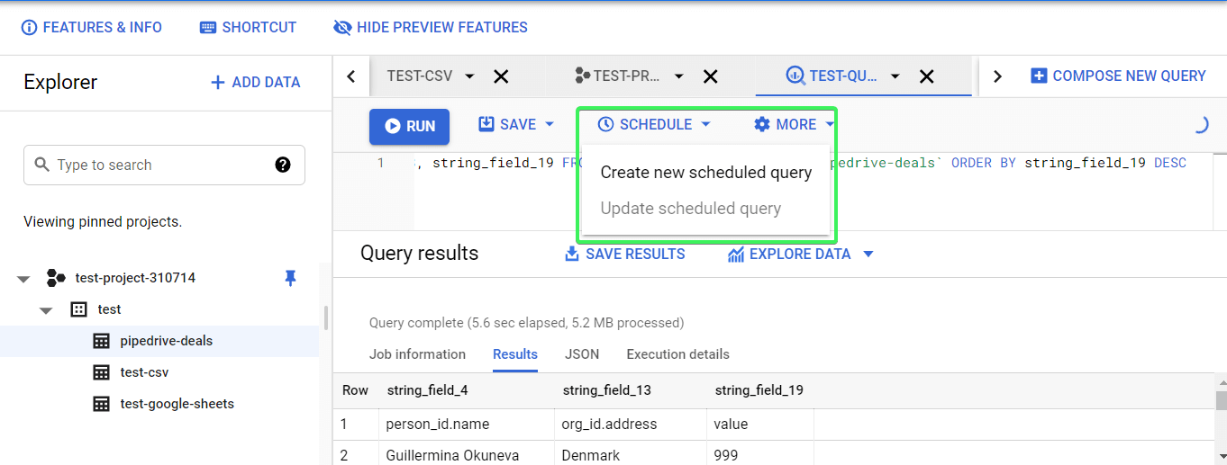
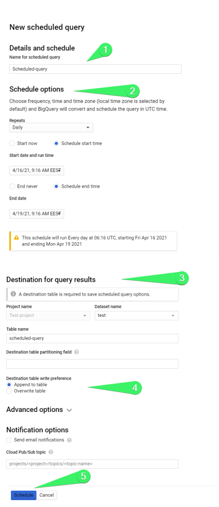
Click Create new scheduled query and define the following parameters:

• Name for scheduled query
• Schedule options
  • Repeats
  • Start date and run time
  • End date
• Destination
  • Table name
  • Write preference (overwrite or append)
    • Overwrite – query results will overwrite the data in the table
    • Append – query results will be appended to the data in the table

Optionally, you can set up advanced options and notification options. Click Schedule when the setup is complete.

Next, you’ll need to select your Google account to continue to BigQuery Data Transfer Service.  

Query history

Let’s say you forgot to save your advanced query, but you want to restore it now. No worries, BigQuery provides you with logs of the queries and jobs you made. You will find them in the popup tabs Jobs history and Query history.

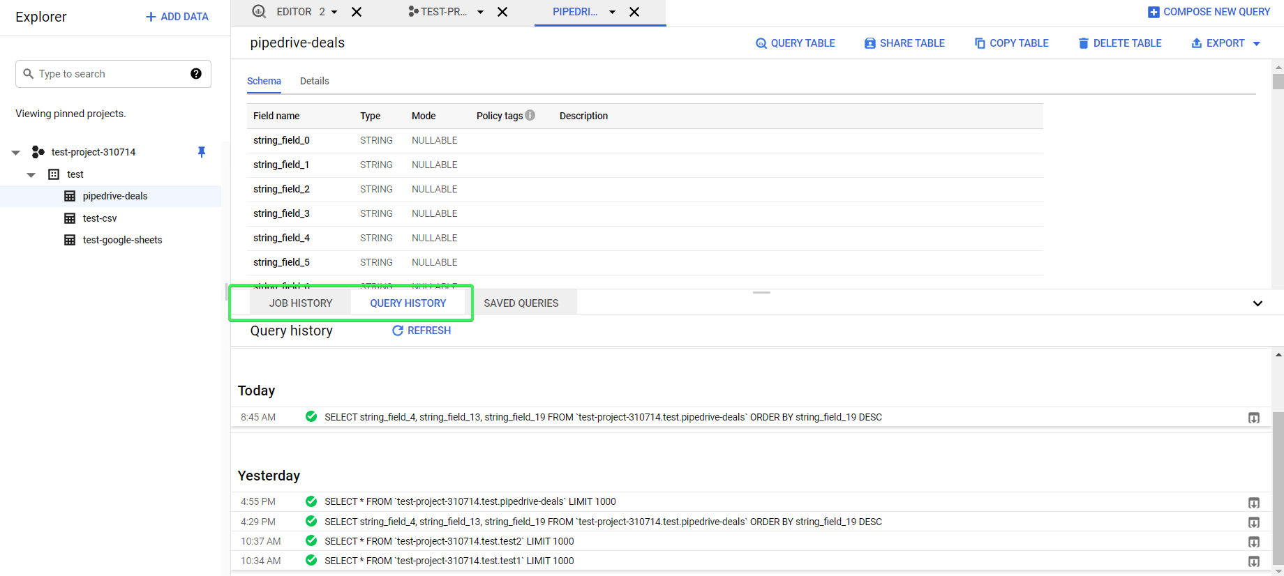
Note: BigQuery displays all load, export, copy, and query jobs for the past 6 months. It limits the job and query histories to 1,000 entries.

Export queries from BigQuery manually and automatically 

In most cases, users need to export the results of their queries outside BigQuery. The common destinations are spreadsheet apps, such as Google Sheets and Excel, visualization and dashboarding tools, such as Google Data Studio (we have a wonderful Google Data Studio tutorial on our blog) and Tableau, and other software. You can also connect Power BI to BigQuery.

BigQuery exporting limits

To open the native BigQuery export data options, you need to click the Save Results button and select one of the following:

• CSV file
  • Download to your device (up to 16K rows)
  • Download to Google Drive (up to 1GB)
• JSON file
  • Download to your device (up to 16K rows)
  • Download to Google Drive (up to 1GB)
• BigQuery table
• Google Sheets (up to 16K rows)
• Copy to clipboard (up to 16K rows)

Read more about BigQuery data export.

Example of exporting query from BigQuery

As an example, let’s choose the BigQuery table option. You’ll need to choose the Project and Dataset, as well as name your table. 

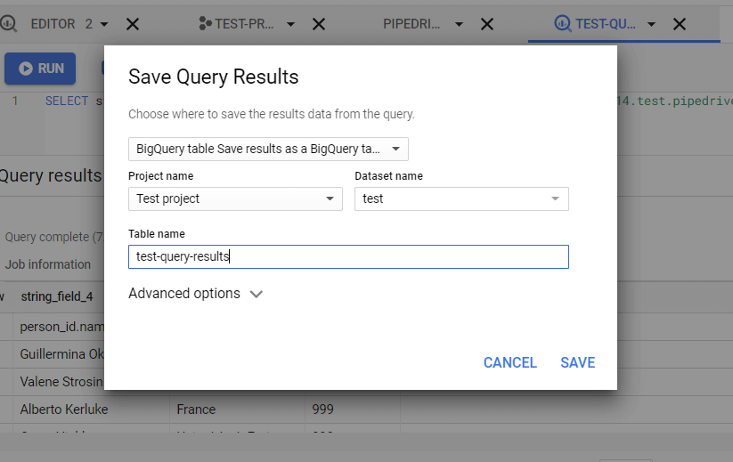
Click Save, and there you go!

Export queries from BigQuery to Google Sheets automatically

Saving your query results to Google Sheets manually is not particularly efficient, especially if you need to do this recurrently. You should automate exporting queries from BigQuery to Google Sheets – with Coupler.io, it only takes a few minutes, and no coding skills are required. 

1. Collect data

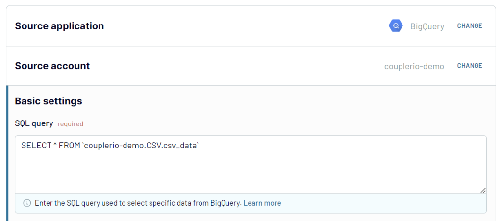
Use the form below to start importing your data by clicking Proceed:

• Connect your BigQuery account and enter your query.

2. Organize and transform data

In the next step, you can check your data and make edits. For example, you can:

• Hide, rename, and rearrange columns.
• Add new columns.
• Split and merge columns.
• Use formulas and perform calculations.
• Blend data from several accounts or sources into one dataset.
• Sort and filter data.

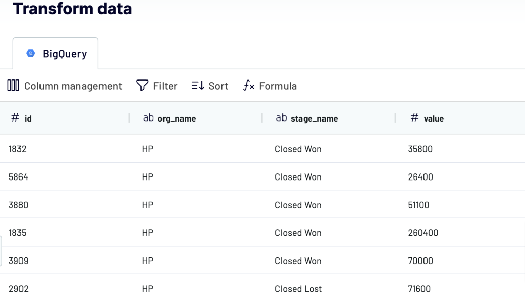
Then, click Proceed.

3. Set up the destination

Connect your Google account. Then, choose a spreadsheet and sheet to export your query results to.

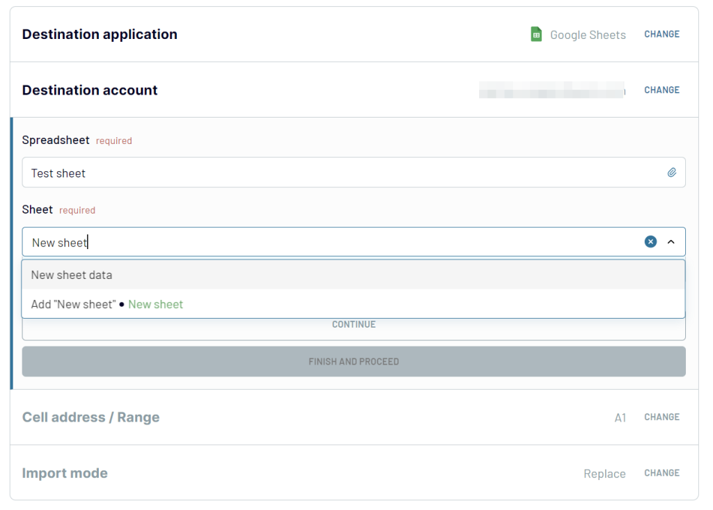
 Turn on the Automatic data refresh and choose the schedule for updates.

Once you’re ready, click Run Importer to get your query results into the spreadsheet.

Coupler.io provides a BigQuery integration that allows you to copy BigQuery table to another table, as well as export queries out of BigQuery.

Automate data export with Coupler.io

Get started for free

How BigQuery stores data

Unlike traditional relational databases that store data row by row, BigQuery’s storage is column by column. This means that a separate file block is used to store each column. This columnar format, called Capacitor, allows BigQuery to achieve a very high throughput, which is crucial for online analytical processing.

BigQuery architecture

In BigQuery’s serverless architecture, the resources for storage and computing are decoupled. This allows you to get your data of any size into the warehouse and get on with data analysis right away. Here are the infrastructure technologies that make this happen:

• Colossus – responsible for storage. This is a global storage system optimized for reading large amounts of structured data, as well as handling replication, recovery, and distributed management.

• Dremel – responsible for computing. This is a multi-tenant cluster that turns SQL queries into execution trees. These trees have leaves called slots, and a single user can get thousands of slots to run their queries.

• Jupiter – responsible for data movement between storage (Colossus) and compute (Dremel). This is a petabit network, which moves data from one place to another, and does so very quickly.

• Borg – responsible for the allocation of hardware resources. This is a cluster management system to run hundreds of thousands of jobs in BigQuery.

How much does BigQuery cost?

Two major variables affect the cost to the end-user:

• Analysis pricing: This involves expenses incurred for executing SQL commands, user-defined functions, Data Manipulation Language (DML), and Data Definition Language (DDL) statements in BigQuery tables. 
• Storage pricing: The amount of data stored in BigQuery determines the cost of storage.

Storage cost

Query cost

– Charges are usually incurred monthly for data stored in BigQuery tables or partitions that are active – meaning that they have been modified in the last 90 days.  – If you haven’t made any changes to your BigQuery tables or partitions in the last 90 days, you may be eligible for a fee reduction of up to 50%. – Charges may apply depending on the amount of incoming data when utilizing the BigQuery storage APIs. – Users pay for each 200MB of streaming data consumed by Google BigQuery.

– With on-demand pricing, you are charged based on the amount of data processed by your queries. You are not charged for failed queries or queries loaded from the cache. Besides, the first 1 TB of query data processed per month is free. Additionally, prices vary by region. – With flat-rate pricing, you pay a fixed charge regardless of the amount of data scanned by your queries. This price option is ideal for clients who need a predictable monthly cost within a specific budget. Users must purchase BigQuery slots to take advantage of flat-rate pricing—more on that soon.

Cost of storing data in BigQuery

Storage cost refers to the cost of storing data in BigQuery. You pay for both active and long-term storage.

• Active storage: Any table or partition of a table that has been updated in the past 90 days is considered active storage. At the moment, BigQuery charges a fixed monthly fee of $0.02 per GiB per month for active logical storage. The active physical storage costs $0.04 per GiB per month. The first 10 GiB is free each month.
• Long-term storage: Any table or partition of a table that has not been updated in the last 90 days is considered long-term storage. After 90 days, the price of storage data decreases by 50%. The price for long-term logical storage is $0.01 per GiB per month. Long-term physical storage will cost more – $0.02 per GiB per month. The first 10 GiB is free each month.

Active and long-term storage are equivalent in terms of performance, durability, and availability. 

You’re charged based on the amount of data you put into BigQuery. To determine the total amount of your data, you must know how many bytes each column’s data type contains. This is the size of BigQuery data types:

Data type	Size
INT64	8 bytes
FLOAT	8 bytes
NUMERIC	16 bytes
Bool	1 byte
STRING	2 bytes
Date	8 bytes
Datetime	8 bytes
Time	8 bytes
Timestamp	8 bytes
Interval	16 bytes

 BigQuery cost per 1 GiB

Type of storage	Price	Free tier
Active logical storage	$0.02 per GiB	The first 10 GiB are free each month
Active physical storage	$0.04 per GiB	The first 10 GiB are free each month
Long-term logical storage	$0.01 per GiB	The first 10 GiB are free each month
Long-term physical storage	$0.02 per GiB	The first 10 GiB are free each month

It costs $0.02 per GiB per month for BigQuery to keep your data in active storage. Thus, if we keep a 200GiB table for one month, the cost will be (200 x 0.02) = $4.

Note: With the free 10GiB every month, a user will get a total of 210GiB for $4.

When it comes to long-term storage, the cost is much lower than with active storage. For example, long-term storage of a 200GB table for one month will cost (200 x 0.01) = $2. If the table is updated, it becomes active storage and the 90-day period resets and starts from the beginning again.

Also, it is important to note that the price of storage varies by location. For example, selecting Mumbai (asia-south1) as a storage location costs $0.023 per GiB, while using the US (multi-regional) (us) or EU (multi-region) (europe) costs $0.02 per GiB.

BigQuery cost per 1 TB

The size of your saved data and the data processed by your queries is measured in gibibytes (GiB). 1 GiB is 2³⁰ bytes or 1,024 MiB. 1 TiB (tebibyte) is 2⁴⁰ bytes or 1,024 GiB.

If a GiB of storage costs $0.02 and 1TB is approximately 1,000 GiB (931.323) then 1TB costs $20.

Note: The cost of data changes from location to location. For active storage, the cost of the data is $0.02 and for long-term storage, it is $0.01.

Let’s say you have 5TB worth of Hubspot data that you would like to import into BigQuery. You can do it automatically with Coupler.io and its HubSpot to BigQuery integration.

To get the cost of 5TB, we will simply multiply the data amount by 1,000 (to convert to GiB), then multiply the result by $0.02 per GB.

5 TB  * 1000 = 5,000 GiB

5,000 GiB * $0.02 = $100

Query price analysis structure in Google BigQuery

We use analytical pricing in BigQuery to calculate the cost to perform queries, including SQL queries, user-defined functions, and scripts, as well as storage pricing to calculate the cost of storing data that you load into BigQuery.

BigQuery has two distinct price levels for its users to select from when executing queries. The price levels are:

• On-demand pricing: In on-demand pricing, you pay based on the size of each query and the number of bytes handled by each query. If the query fails, you will not be charged. The first terabyte of query data processed each month is provided free of charge to all users.
• Flat-rate pricing: Under the flat-rate pricing approach, you pay a set fee regardless of how much data your queries scan. This is the best pricing choice for users who want a consistent monthly fee within a set spending limit. 

Users may access flat-rate pricing by purchasing BigQuery slots, essentially virtual CPUs used by BigQuery to execute SQL queries. The dedicated slot capacity you buy determines the amount of processing power reserved for all of your queries at any given time, rather than for each query separately. If your requests exceed your dedicated capacity, BigQuery queues individual work units and waits for slots to become available. 

As query processing progresses and slots become available, queued work units are dynamically selected for execution, and no additional fees are charged.

Slots are used in both the on-demand and flat-rate pricing, but the flat-rate approach offers you specific control over slots and analytics capacity; for example, in flat-rate pricing, you can choose to reserve slots for: 

• 60 seconds: Flex slots
• Monthly: 30 days
• Yearly:  365 days

Location is important to consider as well.  For example, a monthly cost of $2,000 will give you 100 slots when purchasing from the EU (multi-region), but in London (europe-west2) 100 slots will cost a monthly fee of $2,500. So the number of slots and cost on either of the plans are determined by location.

You can always mix and match the two models to meet your specific requirements. You pay for what you consume with on-demand pricing while with flat-rate pricing, you get an assured capacity at a reduced cost in exchange for a longer-term plan.

BigQuery cost analysis

Now that you know how much specific BigQuery operations will cost depending on your needs, the next step would be to estimate your expenses for those activities. BigQuery cost analysis begins with calculating your query and storage cost to determine your overall expenses.

How to check Google Bigquery query cost

You may use one of the following techniques as a BigQuery cost estimator to evaluate expenses before executing a query:

• Use the query validator in the cloud console: The query validator is located in the BigQuery console and it shows how many bytes of queries it will process.

• Use the —dry run option in the BigQuery command-line tool: You can use the —dry run flag to estimate the number of bytes read when using the bq command-line tool. You can use —dry run when working with API or client libraries. To run, use the —dry run flag with the bq command-line tool.

bq query \
--use_legacy_sql=false \
--dry_run \
'SELECT
  COUNTRY,
  STATE

FROM
  `project_id`.dataset.shipping
LIMIT
  1000'

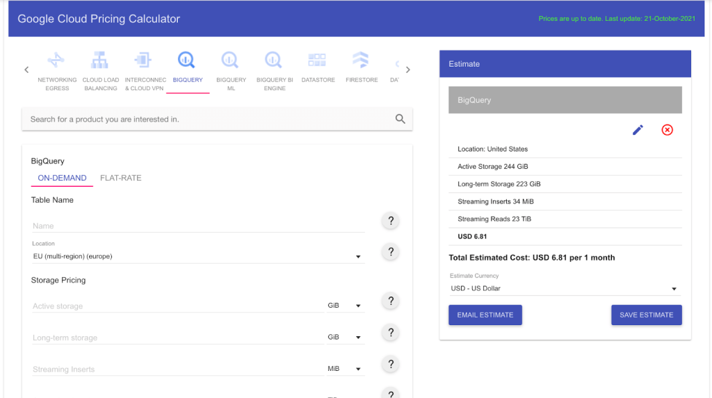
• Use the Google Cloud Pricing (GCP) Calculator: Google offers a price calculator to help you estimate how much money you’ll spend on the resources you might need.

How to estimate using the BigQuery cost calculator

On-demand pricing:

The following steps outline how to estimate your Google BigQuery costs using the GCP pricing calculator for clients with the on-demand pricing model:

• Go to the main page of your BigQuery console.
• When you enter a query, the query validator (the green tick) verifies it and estimates how many bytes it will process.

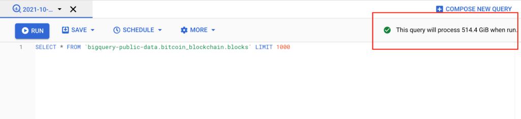
As you can see, this query will use approximately 514.4 GiB.

• The next step is to access the GCP Pricing Calculator. 
• Choose BigQuery as your product and on-demand pricing as your pricing method.
• Complete the on-screen form with all the necessary information, as shown in the picture below.

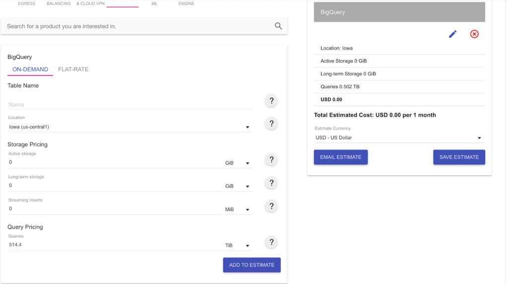
Because we haven’t used up our 1TB free tier for the month yet, the charges to execute our query of 514.4GiB are nothing. However, if you need to run this query every day for the next month, you will use 514.4 * 30 = 15,432 GiB; this will quickly put us about the 1TB free tier.

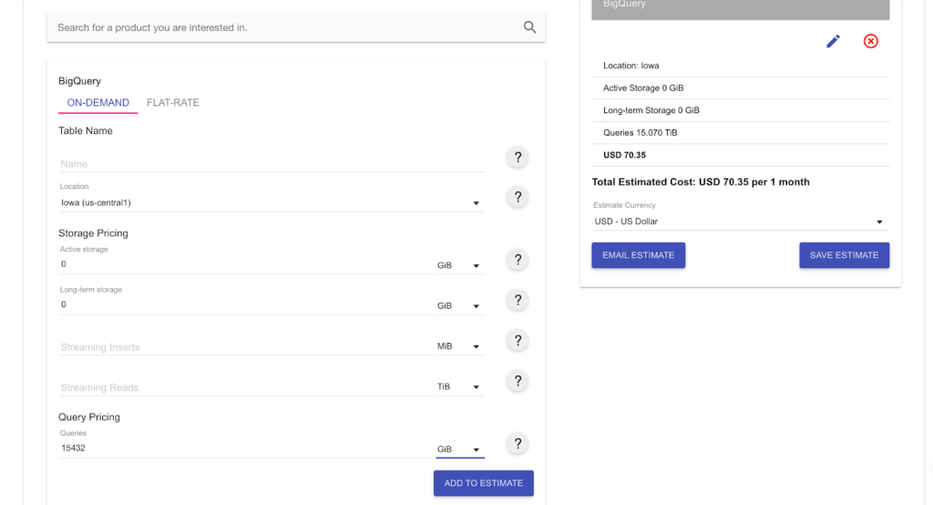
Our total charge now will be $70.35 per month.

Flat-rate pricing:

In flat-rate pricing, you are not billed for bytes processed; rather the queries you run are billed based on your purchased slot. In the example below, we bought 100 slots at the estimated cost of $2,000. Within this limit, we will process the 514.4GiB-worth of queries at no additional charge.

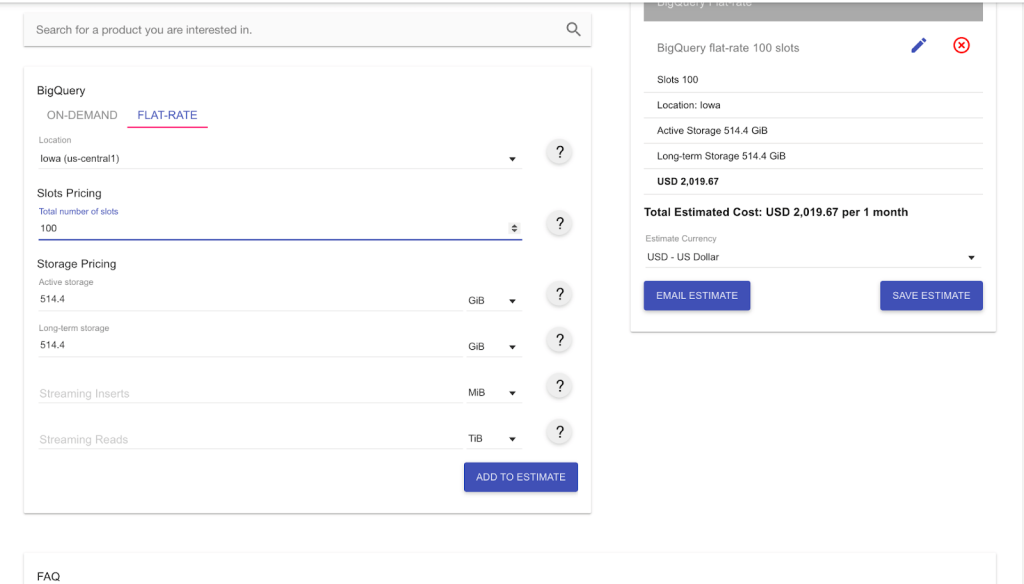
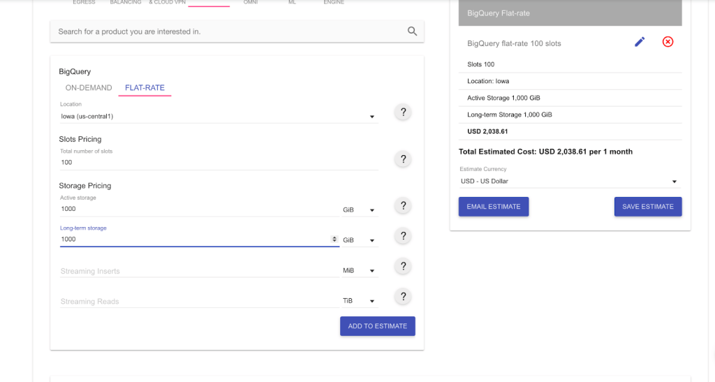
If you send a heavier load of queries, let’s say 1,000 GiB, with the same capacity of 100 slots, the pricing won’t change. You will still only pay $2,000 for the slots you have purchased. 

The query processing may take a bit longer, though. If the available slots are insufficient to process a given query, the query will be queued and processed later when slots are available.

The slot capacity you’ve purchased determines the maximum capacity split among all your queries, rather than the processing power for each query separately.

The estimated cost offered by the tools above may differ from the actual expenses for the following reasons:

• A query clause that performs data filtering, like a WHERE clause, may substantially decrease the amount of data read.
• After the estimate is given, additional or deleted data may increase or reduce the number of bytes read when the query is performed.

How to estimate BigQuery storage and query costs?

To calculate BigQuery storage and query cost, we start by collecting the necessary information to estimate our costs:

• Number of Users 
• Number of Queries 
• Average Data Usage 

As an example, imagine we have a dataset that is used by 10 users per day, each running five queries per day, with an average data usage of 2 GiB per query. We calculate the cost per month, which we’ll assume has 30 days. 

We can then take those parameters and apply a basic calculation to estimate our average monthly cost with BigQuery. 

MONTHLY QUERY DATA USED = 10 * 5 * 2GB * 30 = 3,000 GiB = 3TB 

To calculate the BigQuery storage price, with query data of 3TB per month, as of the time of writing 1TB is around $20 (the exact price depends on the region chosen). So we simply multiply 3TB by the $20 to get the storage cost per month.

3 * 20 = $60

To calculate on-demand query pricing, using the same query data, the price of 1TB is $5. So we simply multiply 3TB by $5 to get the on-demand query price per month.

3 * 5 = $15

The price may decrease if you haven’t used the 1TB added to your account for free each month.

How much does it cost to process 1TB in BigQuery?

For on-demand query pricing, 1TB costs $6.25.

How much does it cost to run a 12 GiB query in BigQuery?

12GiB is approximately 0.01288 TB. Since 1TB costs $6.25, 12 GiB will cost:

6.25 * 0.01288 = $0.08

How much does it cost to run a 100GB query in BigQuery?

100GB is approximately 0.107 TB. To find out how much it costs to run 100GB, we make the following calculation:

6.25 * 0.107 = $0.66

Do views cost extra in BigQuery?

No. Virtual tables are defined by SQL queries as views. In the same manner that you can query a table, you can do the same with views. 

Views may only provide data from the tables and fields that are explicitly requested by the user when queried. The total quantity of data in all table fields referred to directly or indirectly by the top-level query determines how much a query will cost to execute. 

There is no fee for adding or removing a view.

hared pool nor the throughput you will experience is guaranteed by BigQuery. Dedicated slots for running load tasks are also available for purchase.

What is the cost of BigQuery API?

The pricing model for the Storage Read API is on-demand pricing. On-demand pricing is entirely usage-based, with all customers receiving a complimentary tier of 300TB per month. 

However, you will be charged on a per-data-read basis on bytes from temporary tables as they are not considered part of the 300TB free tier. Even if a ReadRows function fails, you pay for all of the data read during a read session.

If you cancel a ReadRows request before the stream’s conclusion, you will be billed for any data read before the cancellation.

Bonus: What is BigQuery ML?

Do you know that SQL can be used for machine learning? Well, it’s true! BigQuery ML lets anyone do this using SQL. You can create and train a model without ever exporting data out of BigQuery! So, don’t worry if you can’t code in Python, R, or other programming languages for ML. With just SQL, you can still build and train a machine learning model.

Simply put, Google BigQuery ML (BQML) is a set of SQL extensions to support machine learning. It was launched in 2018 with the following purposes:

• To empower data analysts and scientists to use machine learning through existing SQL skills and tools. It’s more common to find data analysts with SQL expertise than ones with ML programming backgrounds. So, with BigQuery ML, analysts who are familiar with SQL but can’t code in R, Python, or Java can still build powerful ML models.
• To allow data analysts and scientists to do ML locally inside BigQuery. This means they don’t need to move the data out of the platform, saving time on machine learning development.

BigQuery ML supported model types and algorithms

The terms “model” and “algorithm” are frequently used interchangeably in machine learning, but they’re not the same thing. A machine learning algorithm is the step-by-step instructions run on data to create a machine learning model. So, you can say that a machine learning model is the output of an algorithm.

BigQuery ML supports supervised learning algorithms such as linear and logistic regressions. It also supports unsupervised learning algorithms in that you can use k-means to cluster your data based on similarity. 

As of this writing, BigQuery ML supports the following model types:

BigQuery ML model type	ML problem type and additional note
Linear regression	To solve regression problems. Use LINEAR_REG when the label is a number, for example, to forecast product sales on a certain day.
Logistic regression	You can use LOGISTIC_REG for either BigQuery ML binary logistic or multiclass classification. Use for binary classification when the label is TRUE/FALSE, 1/0, or only two categories, for example, to determine whether a flight will be late or not.  Use for multiclass classification when the label is in a fixed set of strings, for example, to classify whether an email is a primary, social, promotions, updates, or forums.
Deep Neural Network (DNN)	To create TensorFlow-based DNN for solving regression and classification problems. Use DNN_REGRESSOR for regression problems. Use DNN_CLASSIFIER for binary and multiclass classification problems.
Boosted Tree	For creating “boosted” decision trees, which have better performance than decision trees on extensive datasets. You can use boosted tree models for classification and regression problems.  Use BOOSTED_TREE_REGRESSOR for regression. Use BOOSTED_TREE_CLASSIFIER for binary and multiclass classification problems.
Matrix factorization	For creating a recommendation system, for example, to recommend the “next” product to buy to a customer based on their past purchases, historical behavior, and product ratings.
K-means	Use it when labels are unavailable, for example, to perform customer segmentation.
Autoencoder	You can use it to detect anomalies in your data.
Time series	BigQuery ML for time series is popular for estimating future demands, such as retail sales or manufacturing production forecasts. It also automatically detects and corrects for anomalies, seasonality, and holiday effects.
AutoML tables	You can use AutoML for any regression, classification, and time series forecasting problems. It will automatically search through various models and find the best one for you.
TensorFlow model importing	Use it if you have previously trained TensorFlow models and want to import them to BigQuery ML to perform predictions on them.

BigQuery ML built-in vs. external model types

Based on where the models are trained, the model types listed above can be classified into two different categories:

• Built-in models, which are built and trained within BigQuery. These include linear regression, logistic regression, k-means, matrix factorization, and time series models. 
• External models (custom models), which are trained outside BigQuery. Examples include AutoML Table, DNN, and boosted tree models trained on Vertex AI.

Built-in models can be trained very quickly. You can get high-quality models with external models, but they’ll take longer to train—it can be hours or even days. Choosing a built-in vs. external model will also be different in pricing.

BigQuery ML example

In this example, we’ll use the BigQuery public dataset chicago_taxi_trips to build a model to predict the taxi fares of Chicago cabs. The label we’re going to predict is the trip_total, which is the total cost of the trip. We’ll use a linear regression model, the simplest regression model that BigQuery ML supports. 

The prediction we’re going to make is based on these three attributes also called features:

• trip_seconds (time of the trip in seconds) 
• trip_miles (distance of the trip in miles)
• company (the taxi company) 

Note: Before choosing the input features of our ML models, it’s best to do more analysis to verify that those features do in fact influence the label. Deciding which features to include in a machine learning model is called feature engineering, and it is often considered the most important part of building an accurate machine learning model. In this example, however, let’s just pick those three features for simplicity.

This is the step-by-step guide for this example:

• Create a dataset
• Create a linear regression model using the CREATE MODEL statement
• Evaluate the model using the ML.EVALUATE function 
• Make a prediction using the ML.PREDICT function
• Generate batch predictions

Create a dataset

Now let’s first create a BigQuery dataset to store our ML model by following the steps below:

Step 1: Go to the BigQuery page.

Step 2: In the toolbar, select your project (or create a new one).

Step 3: In the Explorer, expand the View actions icon () next to the project, then select Create dataset.

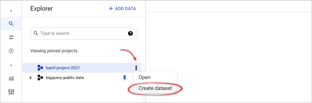
Step 4: On the Create dataset pane, enter a unique Dataset ID, for example, bqml_example. You can leave the other options as default, then click CREATE DATASET. 

Create model using BigQuery ML

Next, let’s create a linear regression model and save it into the bqml_example dataset we created previously. Here are the steps to create the model using the CREATE MODEL statement:

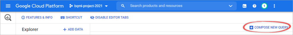
Step 1: Click the COMPOSE NEW QUERY button.

Step 2: Write the following SQL query in the editor.

CREATE OR REPLACE MODEL bqml_example.chicago_taxi_trip_model
OPTIONS (input_label_cols=['trip_total'], model_type='linear_reg') AS
SELECT  trip_seconds, 
        trip_miles, 
        company,
        trip_total        
FROM    `bigquery-public-data`.chicago_taxi_trips.taxi_trips
WHERE   trip_seconds BETWEEN 60 AND 7200
        AND trip_miles > 0
        AND fare >= 3.25
        AND company IS NOT NULL;

Query explanation:

The above SQL creates and trains a model named chicago_taxi_trip_model and saves it in the bqml_example dataset. The model uses data from the taxi_trips table in the chicago_taxi_trips dataset under the bigquery-public-data project.

Notice that the input label column and model type are specified in OPTIONS. Because the label is numeric, we use linear_reg model type as already discussed in the previous section about BigQuery ML supported model types. 

In the WHERE clause, we can put filters to exclude certain data in our training. For example, it’s very rare for a person to be in a taxi for under 1 minute or more than 2 hours. In this case, we also exclude trips with fares under $3.25, zero mile distance, and no information about taxi company names.

Step 3: Click RUN.

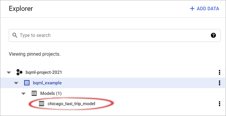
The query takes about 4 minutes to complete. After that, the new model chicago_taxi_trip_model appears in the navigation panel. 

Evaluate BigQuery ML model

We can get the evaluation results by running the following SQL query:

SELECT * FROM ML.EVALUATE(MODEL bqml_example.chicago_taxi_trip_model)

Result:

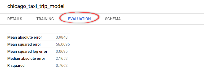
As you can see from the above screenshot, the mean absolute error value is about $3.98. This means that you should expect to predict the taxi fare with an average error of about $3.98. 

Note: To see the evaluation results, alternatively, you can click chicago_taxi_trip_model in the left panel. You will see several tabs containing info about this model. One of them is the Evaluation tab, where you can view the evaluation summary.

Predict with the BigQuery ML model 

We can try out the prediction by passing in a row for which to predict. For example, to get the predicted Chicago Taxicab total fare for a trip with 1.5 miles and 10 minutes, we can use the following code:

SELECT * FROM ML.PREDICT(MODEL bqml_example.chicago_taxi_trip_model, 
  (SELECT 600 as trip_seconds, 1.5 AS trip_miles, 'Chicago Taxicab' as company) 
)

Result:

As you can see, the predicted total fare is about $13.49. Because we have a mean absolute error of $3.98, the actual fare is expected to be in the range of $9.38 to $17.47.

Generate batch prediction via Google BigQuery ML 

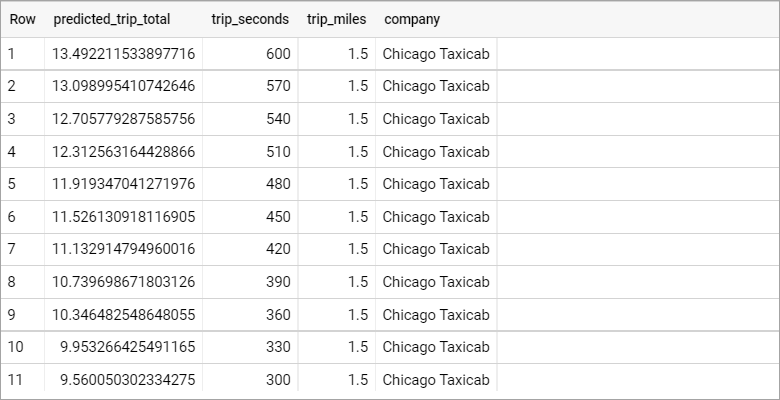
We can also predict many rows at once. For example, here we’re going to predict the cab fare for trips with a duration every 30 seconds between 300 to 600 seconds using array generation:

WITH time_seconds AS (
  SELECT GENERATE_ARRAY(300, 600, 30) AS seconds
)
SELECT * FROM ML.PREDICT(MODEL bqml_example.chicago_taxi_trip_model, 
  (SELECT t_seconds AS trip_seconds, 1.5 AS trip_miles, 'Chicago Taxicab' as company
  FROM time_seconds, UNNEST(seconds) as t_seconds) 
) 
ORDER BY trip_seconds DESC;

The query returns 11 rows, sorted from longest to shortest trip duration:

BigQuery ML Geography data types

As a data warehouse, BigQuery can store data of many types: numeric, date, text, geospatial data, etc. Learn more about Google BigQuery data types. 

When you want to provide geolocation for your model input, using the state or country name might not give you enough detail, so it doesn’t work well in some cases. It’s recommended to use precise locations. However, using a WKT representation (e.g., POINT(-122.35 47.62)) or GeoJSON (e.g., { "type": "Point", "coordinates": [-122.35, 47.62] }) is not recommended either.

A better choice is using a GeoHash representation, a hash string representation of a geographic location. The longer the shared prefix between two hashes, the closer together they are spatially. 

To get a GeoHash representation of a location, use ST_GeoHash function in BigQuery.

Example: Adding locations as inputs to our model

Now, let’s add the pick-up and drop-off locations and use those as additional inputs to our model. We’ll create a new model and name it chicago_taxi_trip_geo_model.

CREATE OR REPLACE MODEL bqml_example.chicago_taxi_trip_geo_model
OPTIONS (input_label_cols=['trip_total'], model_type='linear_reg') AS
SELECT  trip_seconds, 
        trip_miles, 
        company,
        ST_GeoHash(ST_GeogPoint(pickup_latitude,pickup_longitude), 5) as pickup_location, 
        ST_GeoHash(ST_GeogPoint(dropoff_latitude,dropoff_longitude), 5) as dropoff_location, 
        trip_total        
FROM    `bigquery-public-data`.chicago_taxi_trips.taxi_trips
WHERE   trip_seconds BETWEEN 60 AND 7200
        AND trip_miles > 0
        AND fare >= 3.25
        AND pickup_latitude IS NOT NULL AND pickup_longitude IS NOT NULL
        AND dropoff_latitude IS NOT NULL AND dropoff_longitude IS NOT NULL
        AND company IS NOT NULL;

After that, run the following query to get the evaluation results:

SELECT * FROM ML.EVALUATE(MODEL bqml_example.chicago_taxi_trip_geo_model)

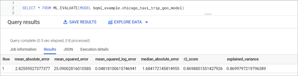
As you can see, this model results in a mean absolute error of about $2.83, a significant improvement over the $3.98 we got from the previous model. We can conclude that pick-up and drop-off locations also affect the taxi fare.

BQML pricing

When you use BigQuery ML, your training data and ML models are stored inside BigQuery. You will be charged mainly for storage and queries. The pricing for queries will also be differentiated into queries for analysis and CREATE MODEL statements—see the following table:

Resource	Detail
Storage	The first 10 GB BigQuery storage per month is free.   After that, you’ll be charged $0.020 per GB of data stored in BigQuery. This price automatically drops by approximately 50% if you don’t make any modifications to your data for 90 consecutive days.
Queries (analysis)	The first 1 TB of data processed by queries that use BigQuery ML functions (ML.PREDICT, ML.EVALUATE, etc.) is free. After that, you will be charged $5.00 per TB.
Queries (CREATE MODEL)	For built-in model types: The first 10 GB of data processed by queries that contain CREATE MODEL statements per month is free. After that, the price is $250.00 per TB.  For external model types: The price is $5.00 per TB, plus Vertex AI training cost.

Note: The above pricing applies if you use BigQuery on-demand pricing. But if you are a flat-rate customer, BigQuery ML costs are included in your BigQuery monthly payment ($2,000 per month, or lower if you choose a longer-term commitment).

Learn more about BigQuery

Let’s be honest – our goal was not to write a perfect BigQuery tutorial but to provide you with the answers every beginner has when they discover a new tool or technology. We are sure that you’ll probably have more questions after reading it, for example, about the BigQuery cost. Check out our blog – we’ve already covered some questions. However, for others, you’ll have to find the answers to them yourself. 

The premier source of information is the official BigQuery documentation, where you’ll find an extensive knowledge base of BigQuery usage. The drawback of this source is that it’s absolutely huge and sometimes over-structured (as most of Google documentation is).

From our side, we’ll try to cover other BigQuery-related topics to clarify some advanced points like BigQuery SQL syntax or using client libraries to get started with the BigQuery API in your favorite programming language. Good luck!

Zakhar Yung

A content manager at Coupler.io whose key responsibility is to ensure that the readers love our content on the blog. With 5 years of experience as a wordsmith in SaaS, I know how to make texts resonate with readers' queries??