The calculations in Google Sheets are not limited to basic arithmetic operations like extraction, multiplication, and so on. This spreadsheet app provides more options to calculate your data for digital marketing, financial modeling, or statistical analysis. Let us dive right into things and start off by understanding the most basic concept.
How to make calculations in Google Sheets?
Remember how you used to perform math calculations? You can make calculations as easily in Google Sheets using formulas. Formulas in Google Sheets execute calculations on spreadsheet data. You can use formulas for simple calculations like addition and subtraction, as well as more complex ones like wage deductions or test averages.
One of the biggest advantages of using Google Sheets is that its formulas are dynamic, meaning that if you alter the data in the spreadsheet, the result will be recalculated immediately wherever it occurs without you having to re-enter the formula.
How to make calculation rules on Google Sheets
The process of making calculation rules is very simple.
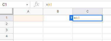
- Click and select the cell you want to display the result in.
- Use the equal sign ‘ = ‘ to start the equation of the calculation.
- Type the cell address of the cell you want to refer to first.
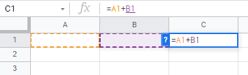
- Use the mathematical operator that you want it to perform, for example ‘+’.
- Type the cell address of the cell you want to refer to second and press enter.
How do I perform simple calculations in Google Sheets?
To perform simple calculations in Google Sheets, first we will create a basic formula. In our sample formula, we will first add numbers 10 and 5 and then subtract 3.
- Type in the following data into the relevant cells.
- A1: 10
- A2: 5
- A3: 3
- Select cell A4 and type an equal sign (=).
Note: In a Google spreadsheet, you should always begin by entering the equal sign in the cell where you wish the answer to appear.
- Following the equal sign, enter
A1+A2-A3.
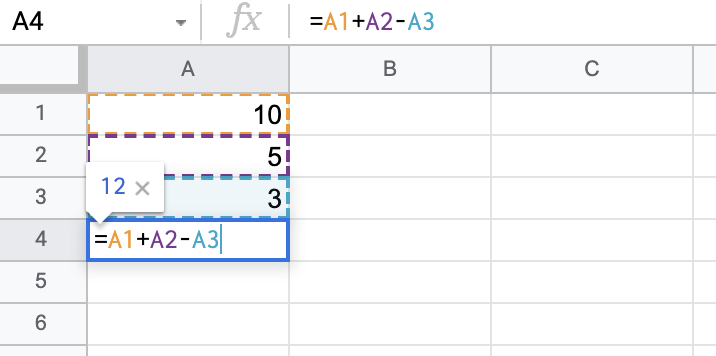
- Press Enter, and you will have your result shown in A4.
Note: By using the cell reference in the formula, the answer will automatically change if there is a change in the values in the cell.
Another way to add cell references is by using a feature known as point and click. This feature allows you to click and select the cell of the data and add its reference to the formula.
How to have Google Sheets repeat a calculation
Most of the time, you have to repeat a calculation or apply your function to multiple rows or columns. And it’s very simple to do it on Google Sheets.
Here are the steps to repeat the calculation:
- Click the cell which contains the formula you want to repeat.
- A dark square will pop up on the bottom right of the cell.
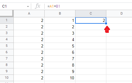
- Click and drag it. Stop at the cell you want to end on.
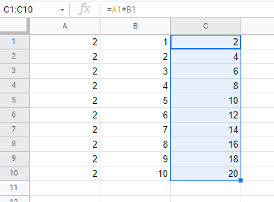
This is the method for beginners who work with small data sets. If you deal with bigger ones, you’d better use ARRAYFORMULA in Google Sheets.
How to make horizontal calculations in Google Sheets
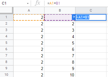
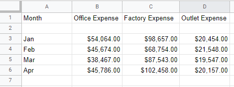
In the last calculation, we just used cells of Column A to perform a vertical calculation. But we can use multiple columns to perform horizontal calculations in Google Sheets. Let’s take an example where we’ve calculated the total expenses of a company.
- We have expenses for the office, factory, and outlet in separate columns.
- To calculate the total expense for each month, we’ll use the SUM formula. Type “ = SUM” and then press the shift key and select all the cells.
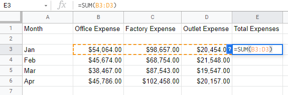
- Press Enter and you will see the total expenses of the company for one month.
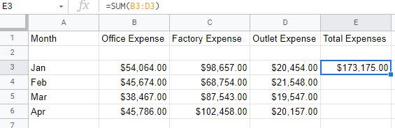
- Now, to repeat the calculation for the other months, just apply the ‘click & drag’ method explained earlier, and you will calculate the total expenses for each month.

The rules for vertical and horizontal calculations are the same in Google Sheets.
Google Sheets percentage calculation
When performing tasks in Google Sheets, you’ll frequently need to use percentages to calculate things like sales tax, test results, inflation rates, and a variety of other things.
Google Sheets makes it plain and simple to calculate and format percentages with a few clicks and a simple formula.
Formatting percentage
You don’t have to multiply the answer with 100 in Google Sheets, simply because you can set the format of the cells to percent, and Google Sheets will do it for you.
- Select the range or cell you want to format.
- Go to Format > Number > Percent in the Google Sheets menu.
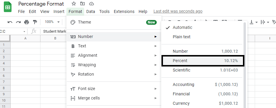
- Click Percent to apply the format.
Google Sheets formula for percentage
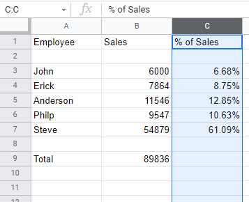
The general formula for percentage is Part/Total. Let’s look at an example where we have to find the percentage of sales for each employee.
- Make a list for employees and another one for sales.
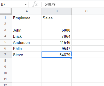
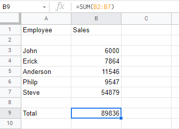
- Get the total amount of sales by adding them all together.
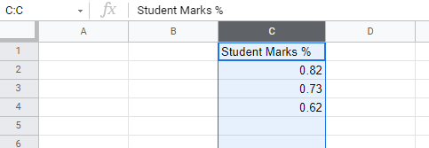
- Now, to find the percentage of sales, use the formula part/total. In this example, we are dividing each employee’s sales cell by the total cell.
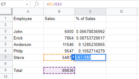
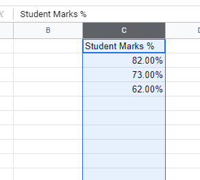
- Notice how the results are in a fraction. We can easily convert them into percentages by using the format.
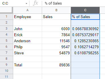
- After applying the format, we can see the percentage of sales of each employee.
How to make part of a cell calculation static in Google Sheets
In Google Sheets, we use cell referencing to assist our calculations in finding the data they require. These values aren’t always set in stone; in fact, they’re not always known when the formulas are applied. Google Sheets will automatically change the cell address in the formula when you are applying it to multiple cells. To overcome this, you have to make the cell static in the formula.
We use absolute referencing to make part of the cell static. You can make one or both characteristics of the cell static using the absolute reference. That is, you can lock the column and/or row. Simply add a “$” before the column or row to accomplish this. Here’s how we go about it:
$A$1 – Makes both column and row static
$A1 – Makes column static
A$1- Makes row static
Google Sheet static calculation
Let’s look at an example to see how to use the absolute reference to do a static calculation.
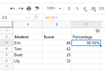
If we try to copy the equation to find the percentage of other students, the formula will automatically adjust. This will be wrong as we want the cell reference of C1 to be static in the equation.
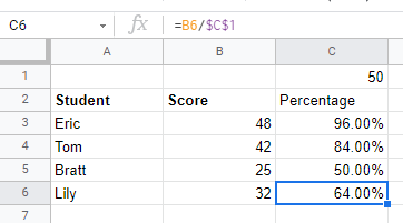
To overcome the problem, we used absolute reference in the formula and made cell C1 static.
How to do an average calculation in Google Sheets
The mean is the most fundamental sort of average. This is what most people mean when they say “average” without explaining what kind of average they’re talking about. As a result, the AVERAGE function in Google Sheets is utilized to calculate the mean.
A function is a formula that Google Sheets runs on your data to perform calculations automatically. You can design a formula that performs computations on data entered in specific cells of the spreadsheet using functions. They provide a quick way to do calculations.
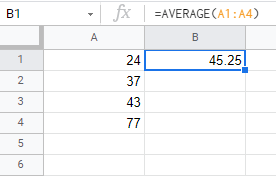
Let’s see how the AVERAGE function is used in Google Sheets.
- Select the cell you want the result of average function in. Type in the average function and select the cells you want the average of.
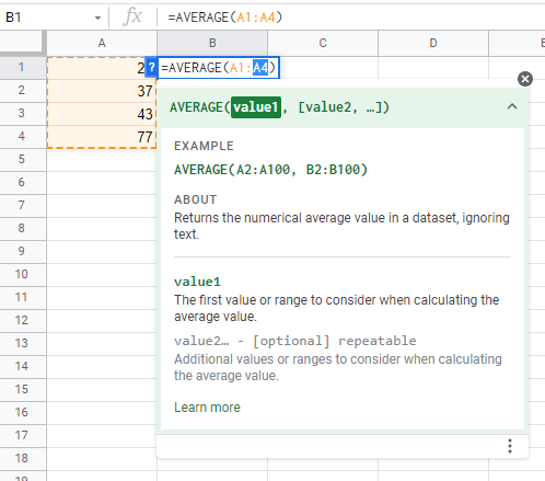
- Press Enter, and you will see the calculated average.
Google Sheets time calculation
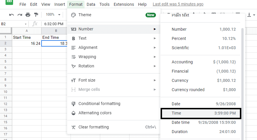
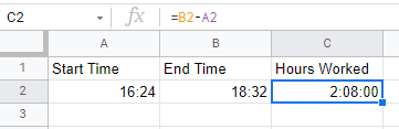
Calculating duration is a common activity for many people who keep track of their work hours on a spreadsheet. Record and time calculation in Google Sheets is very common. It is mostly used to keep track of work hours. However, in order to understand the final duration, the cells must be formatted correctly:
- Select the first column (time in) and the second column (time out) and change their format to Time.
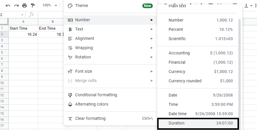
- Change hours worked format to Duration.
- Now calculate the duration by subtracting End time cell B2 from A2.
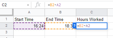
- Press Enter, and you will calculate the hours worked.
The Google Sheets time calculation can be used to calculate age and dates as well.
Google Sheets age calculation
You can calculate the age of a given period in Google Sheets. This can be helpful to keep track of people’s birthdays, contracts, etc.
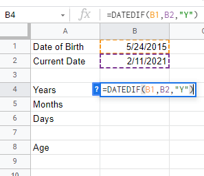
Use Google Sheets DATEDIF function to calculate age. You can use this function to calculate years, months, and days between two dates.
Here are the unit arguments you can use in the DATEDIF function:
- “ Y “ – This calculates the total number of years that have passed between the two dates.
- “ YM “ – This calculates the total number of months between the two dates after the completed years and months.
- “ MD “ – This calculates the total number of days between the two dates after the completed years and months.
Here is how to use the function in Google Sheets.
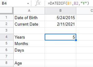
- First, calculate the number of years passed, you do this by using the =DATEDIF(B1,B2,“Y”)
It shows 5 years instead of 6 because 5 full years have passed between the two dates.
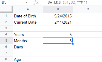
- Then calculate the number of months (not counting the completed years) with the formula
=DATEDIF(B1,B2, "YM")
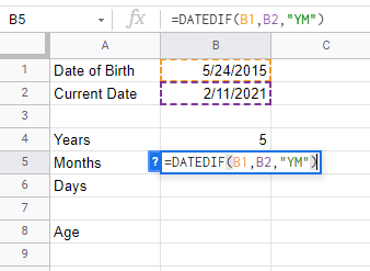
We used the “YM” argument in the formula to calculate the months passed between the two dates after the completed years. In this case, 8 months have passed after 5 years.
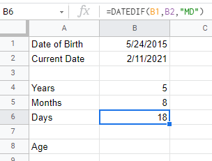
- Last, calculate the remaining days with
=DATEDIF(B1,B2,“MD”)
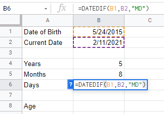
“MD” argument in the formula specifically tells us the days left after the years and months.
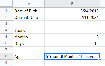
- And if you want to show all the values together, you have to use this formula:
=DATEDIF(B1,B2,"Y")&"Years"&DATEDIF(B1,B2,"YM")&"Months"&DATEDIF(B1,B2,"MD")&"Days"
=SUBSTITUTE(SUBSTITUTE(SUBSTITUTE(
  "{{YEARS}} Years {{MONTHS}} Months {{DAYS}} Days",
  "{{YEARS}}", DATEDIF(B1,B2,"Y")),
  "{{MONTHS}}", DATEDIF(B1,B2,"YM")),
  "{{DAYS}}", DATEDIF(B1,B2,"MD")
The result:
Google Sheets date calculation
You can also calculate the days between two dates to keep track of the duration of projects, loan payment period, etc. To count the days between two days, we use the DAYS function in Google Sheets. The following are the steps to use the DAYS function.
- Make separate columns with date format for Start and End Dates.
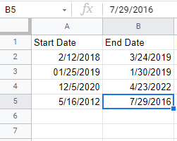
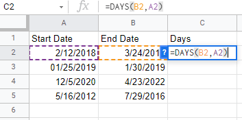
- Make a Days column where you will calculate the days between the two dates. Use the formula
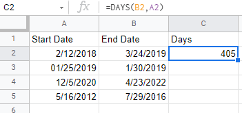
=DAYS(B2,A2)
B2 is the cell address of the ending date.
A2 is the cell address of the starting date.
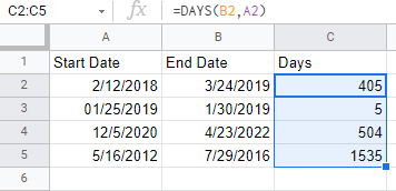
- Press Enter, and you’ll calculate the days between the given dates.
- Apply the formula to other dates.
How to use Power Calculation in Google Sheets
Google Sheets is an excellent tool for storing data and performing calculations. In addition to carrying out simple mathematical operations such as addition and subtraction, it can calculate exponents or power of number Google Sheets.
The easiest way to calculate power or exponent in Google Sheets is to use the power operator. The power operator or Caret is an upside-down V-shaped character on the keyboard and is used inside a formula to calculate exponent quickly. This is how to use it:
- Select the cell you want to store the value of the exponent in and type ” = “.
- Type the base number. For example, type 4 to calculate 4 raise to power 4.
- Type the power operator by holding down the shift key and pressing the 6 key (on a standard United States qwerty keyboard).
- Now type the exponent, in this case, 4.
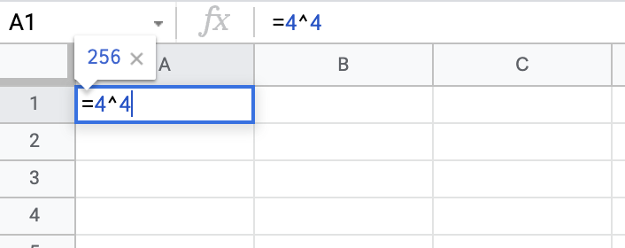
- Press Enter, and your power calculation will be complete, and the result will be displayed.
You can perform the same calculations using reference cells, for example, the formula =A2^A3.
Make your calculations dynamic with automatic data refresh in Google Sheets
Before making calculations in Google Sheets, you need to import data. You can do this via copying and pasting datasets manually or exporting-importing CSV files. However, this can be very time-consuming if you need to refresh the data frequently, like every day. The obvious solution here is to automate data import from your sources to Google Sheets.
You can easily do this with Coupler.io. It’s a reporting automation solution that lets you schedule data exports from 60+ apps and data sources. Moreover, it’s available as a Google Sheets add-on to manage your imports right from your spreadsheet.
You only need to select your source app in the form below and click Proceed.
You’ll be prompted to create a Coupler.io account for free and connect your data source account. Then select the data to load to Google Sheets.
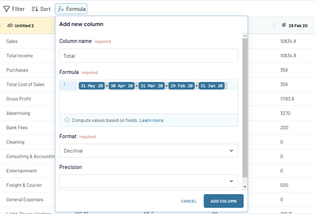
Coupler.io also allows you to perform basic calculations on the go before the data hits your spreadsheet. You can sort and filter records, rename and edit columns, add custom columns, and even blend data from multiple sources.
After that, you need to specify the spreadsheet and the sheet where to load your data. You can even specify an exact range of cells (e.g. B5:G10) for importing data that only fit into this range.
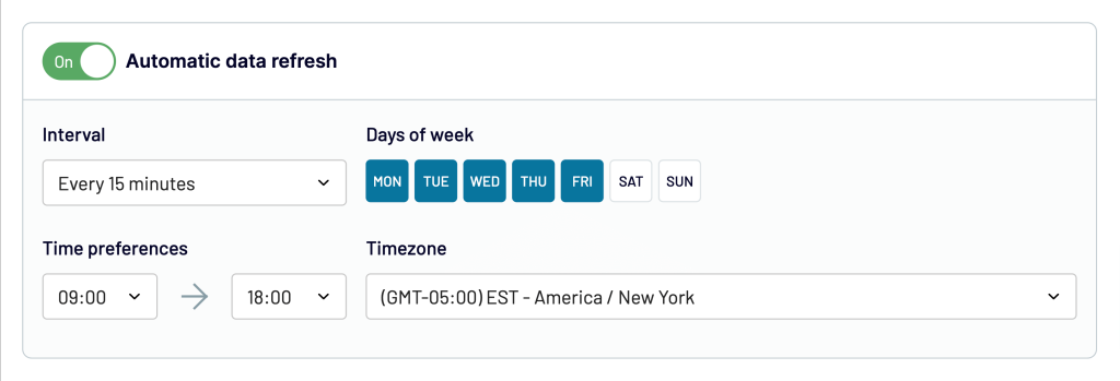
The last step is to enable Automatic data refresh and configure the desired schedule. You can have your data refreshed up to every 15 minutes!
This means that your calculations in Google Sheets will always be up-to-date without any manual effort from your side. Here is what it looks like. We’ve imported inventory data from our Shopify store:
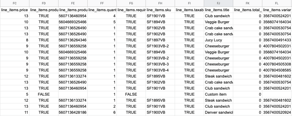
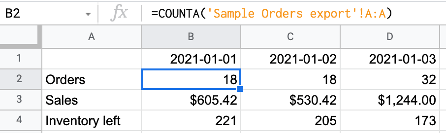
In the spreadsheet, we create a new tab where, for each day, we’ll be automatically calculating:
- Orders received
- Total sales
- Remaining inventory
For the first field, we use the COUNTA formula. It returns the number of rows in the tab with orders that contain any values. So, basically, we get the number of orders we received. To reference a value of another tab, you can type in its name as shown below or simply type in a function name, open the brackets, jump to the desired tab, and select the value you wish to use.
For sales and inventory, we use the common SUM() function that sums up all the numerical values in the selected range.
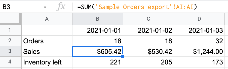
As the importers run every day, the data is automatically calculated in my spreadsheet.
How to get the number from a calculation in Google Sheets
In some cases, you want to remove all the text or strings from a cell value and extract only the numbers from it. Google Sheets have a function that can remove the text and extract numbers.
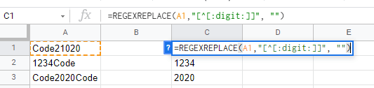
=REGEXREPLACE(A1,"[^[:digit:]]", "")
The arguments of the REGEXREPLACE function are:
Text: The cell address that contains the source or string from which you want to extract the numbers.
Regular_expression: This specifies the part of the string or text that you’re looking for. And to extract numbers from text, we use this [^[:digit:]] regular expression.
Replacement: is the text that will be substituted into the original text.
Let’s put this formula into practice and see how, you can extract the numbers by using this function:
- Click and select the cell in which you want to extract the numbers.
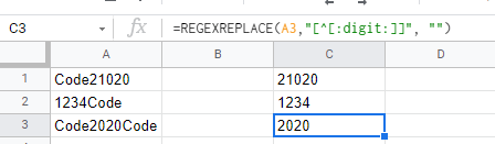
- Type in the formula and press enter. Make make sure you have entered the cell address of the cell you want to extract numbers from.
And here are the results:
Google Sheets iterative calculation
Sometimes when you are repeating complex calculations in Google Sheets, a circular reference error can occur. To overcome this problem, Google Sheets provides a feature called Iterative calculation.
Iterative calculations are calculations that are performed repeatedly until a certain numeric condition is satisfied. Google Sheets uses iterative calculations to obtain formula solutions by repeating the same calculation with previous findings.
It can figure out the possibility of potential solutions by analyzing prior outcomes. There are some calculations that need to be circular, meaning the formula refers to its own cell, either directly or indirectly.
So, if your file contains a circular reference, the formula will become stuck in a loop, calculating over and over again in an attempt to discover a solution.
When iterative calculations are enabled, the Google Sheets file will stop calculating when a set number of rounds have been completed, and the circular formula has discovered a stable result.
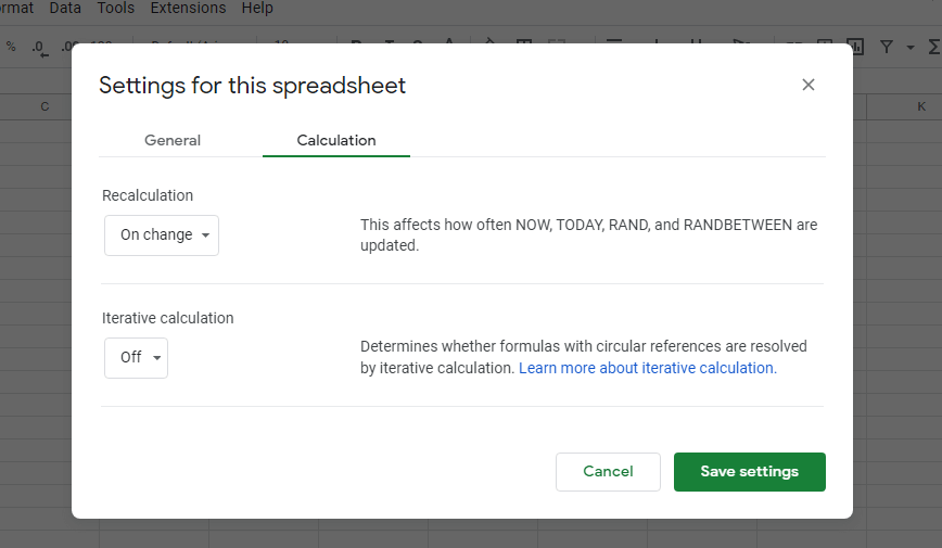
This feature is turned off by default and can be turned on from the settings according to your requirements.
The pathway to the feature is:
File> Spreadsheet settings> Calculation> Iterative Calculation.
Google Sheets loan calculation
Google Sheets provides inbuilt functions to carry out accounting calculations. The PMT function is the one used to perform loan calculations and is available for personal and business use.
The PMT function can be implemented to calculate periodic payments for the loan. The formula syntax is the following:
PMT(rate, number_of_periods, present_value)
- rate: the annual interest rate
- number_of_periods: number of payments to be made
- present_value: the total amount of the loan
Let’s look at an example to see the function in action in this example.
Suppose you took a mortgage loan for your house and the following are the details of it:
- Loan amount: $500,000
- Number of months: 180
- Annual interest rate: 6%
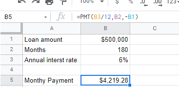
In the function, we divided the rate by 12 because we are paying monthly and we gave a negative value to the loan since we are calculating the amount to pay back.
$4219.28 is the amount you will be paying monthly for 180 months to return the loan.
Google Sheets manual calculation
One fallback of Google Sheets is that it does not allow choosing between automatic or manual calculations. All your calculations are updated automatically on change. The absence of the option to switch between manual and automatic calculation can cause some problems. Since it can automatically change your previous results if you make changes to your formula.
To counter this problem, we recommend you make a copy of your spreadsheet in a new tab and test whatever changes you want to make to the formula. Once you’re satisfied with the outcome, only then should you replace your original tab with the new version.
How to do an if/then calculation in Google Sheets
When working on large spreadsheets, you may find yourself repeating the same calculations for multiple scenarios, but Google Sheets includes excellent tools to help you avoid this extra work. You can use If/Then statements to switch between alternative options if you want to update a Google Sheet when certain conditions are satisfied.
It can help you save a lot of time by eliminating the need to switch between spreadsheets every time something changes.
If/Then statements in Google Sheets refer to the IF function, which returns different values depending on the outcome of a logical test.
The first output used in the logical test is TRUE. The second output is utilized if it is FALSE.
Let’s take a look at how this works in practice:
- Select the cell in which you want the output of the function and type:
=IF(A1=B1, “They are equal, "They are not equal")and press enter.
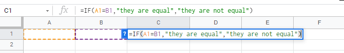
- In this formula, we are setting three parameters. The first statement is the logical test “A1=B1” which will check if the value in these cells is equal or not.
- The second and the third statements are the outputs based on the logical test.
- When the logical test is TRUE, the second parameter is the output.
- When the logical test is FALSE, the third parameter is the resulting output.
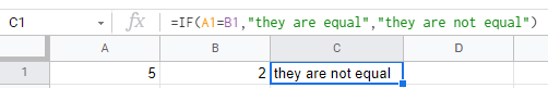
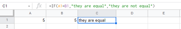
So, whenever you change the values in A1 and B1, the spreadsheet will check the values and report the results accordingly.
Take advantage of the calculations in Google Sheets
Summing up, Google Sheets is a powerful tool that enables you to carry out simple to complex calculations with ease through its inbuilt Google Sheets functions. It allows you to customize calculations to your work requirements, establishing itself as flexible and user-friendly.
To make your calculation dynamic, consider using Coupler.io to automate data exports from your sources to Google Sheets. This way, your calculations will be automatic and your reports will always display the up-to-date. And you won’t have to spend a minute on this.
Automate data import to Google Sheets with Coupler.io
Get started for free