

One of the most common ways people summarize data in Excel is when they are looking for totals based on date criteria – let’s say, to sum values with a specific date, between a certain date range, etc. This article provides various examples of how to sum in Excel by date criteria using SUMIF and SUMIFS.
How to use SUMIF/SUMIFS in Excel with date criteria
We can use both Excel SUMIF and SUMIFS functions to sum values based on date criteria. And here are some important notes when using these functions:
- You can use either SUMIF or SUMIFS if you want to sum by a single criterion. For example, to sum if the date is equal, before, or after a specific date.
- Use Excel SUMIFS date range if you want to sum by multiple criteria, such as to sum if the date is between a certain range.
- Be sure to enclose the date criteria within double quotes (“”).
For the basic usage and syntax of SUMIF and SUMIFS, we’ve already covered that in our previous tutorial: Excel SUMIF function and how to use it. So, if you want a refresher or to see more examples on how to use Excel SUMIF with text criteria or number, feel free to check it out.
Excel SUMIF date range with single criteria examples
Let’s check out some examples on how to sum values based on a single criterion using the SUMIF date range function.
Excel SUMIF: date equals to
In the example below, we are adding up how much was billed for all the tasks that started on June 21, 2023.

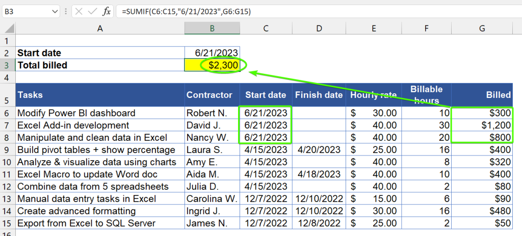
The Excel SUMIF date range formula we use in B3 is:
=SUMIF(C6:C15,"6/21/2023",G6:G15)
The formula sums the amounts in column G (sum range G6:G15) when the date in column C (criteria range C6:C15) is equal to June 21, 2023. Notice that the date criteria is enclosed within double quotes (“6/21/2023”). If it’s not, the formula will return an incorrect result.
You can also use B2 as a cell reference instead of typing the date criteria manually. To do that, just replace “6/21/2023” with B2 (without double quotes):
=SUMIF(C6:C15,B2,G6:G15)
Excel SUMIF: date less than, less than or equal to
In the following example, we calculate how much was billed for tasks that started before April 15, 2023, and on or before April 15, 2023.

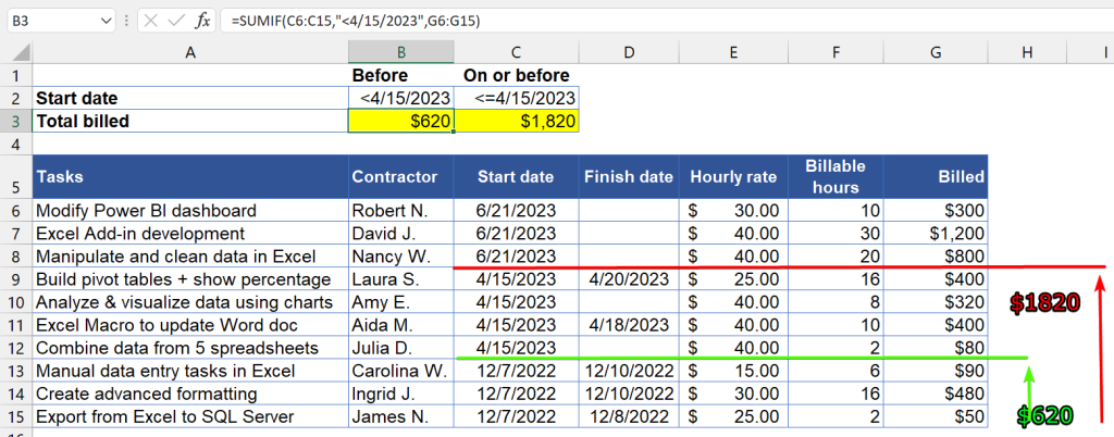
Here are the formulas we use in B3 and C3:
- Before April 15, 2023 (B3):
=SUMIF(C6:C15,"<4/15/2023",G6:G15) - On or before April 15, 2023 (C3):
=SUMIF(C6:C15,"<="&DATE(2023,4,15),G6:G15)
Notice that we use logical operators < for less than and <= for less than or equal to. The formula in C3 shows that we can also use the DATE function in the criteria.
Excel SUMIF: date greater than, greater than or equal to
The following example sums the total bill for the tasks that started after April 15, 2023, and on or after April 15, 2023.

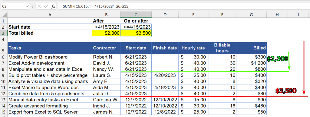
Here are the formulas we use in B3 and C3:
- After April 15, 2023 (B3):
=SUMIF(C6:C15,">4/15/2023",G6:G15) - On or after April 15, 2023 (C3):
=SUMIF(C6:C15,">=4/15/2023",G6:G15)
Notice that we use logical operators > for greater than and <= for greater than or equal to.
Excel SUMIF: date is empty, not empty
The following example shows how to add the total bill for tasks that are not finished yet (finish dates are blank) as well as completed ones (finish dates are not blank).

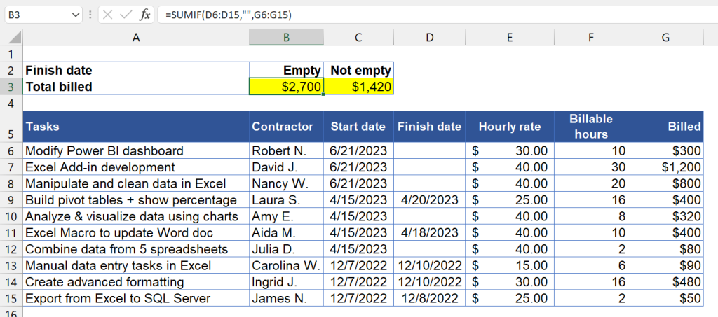
Here are the formulas we use in B3 and C3:
- Finish dates are empty (B3):
=SUMIF(D6:D15,"",G6:G15) - Finish dates are not empty (C3):
=SUMIF(D6:D15,"<>",G6:G15)
Notice that we use the double quotes without any space between ("") to find the dates that are blank or empty. To find dates that are not empty, we use the not equal operator enclosed within double quotes ("<>").
Excel SUMIFS date range with multiple date criteria examples
Now, let’s see some examples of how to sum values based on multiple criteria using the SUMIFS date range function.
Excel SUMIFS between two dates (date range)
The following example sums up the total hours spent for tasks that started between April 15, 2023 and June 21, 2023.

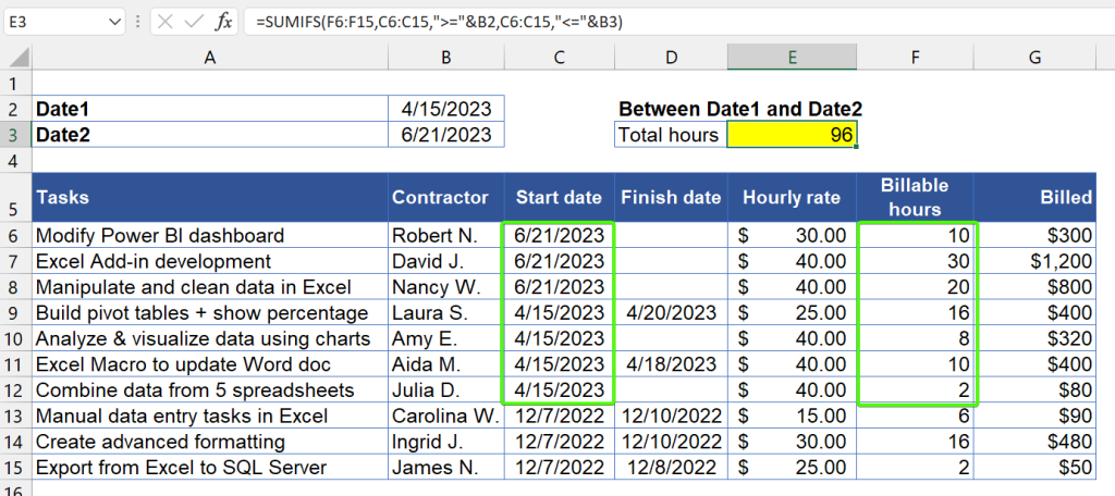
Here’s the Excel SUMIFS date range formula in E3:
=SUMIFS(F6:F15,C6:C15,">="&B2,C6:C15,"<="&B3)
It adds up values in the Billable hours column but only includes rows where the start date is >= B2 (criteria1) and the end date is <= B3 (criteria2), where B2 and B3 refer to "4/15/2023" and "6/21/2023".
Note that we use ampersand for both criteria since we use reference cells. Instead, you can specify the very date in the formula.
C6:C15 works as both the criteria_range1 and criteria_range2.
Excel SUMIF date range from another sheet
What if you want to sum the values that are in another worksheet? For example, you want to get the total billable hours for the data in Sheet1, but your formula is in another sheet.
Summing the total hours from another sheet — here’s the formula in E3:
=SUMIFS(Sheet1!F2:F11,Sheet1!C2:C11,">="&B2,Sheet1!C2:C11,"<="&B3)

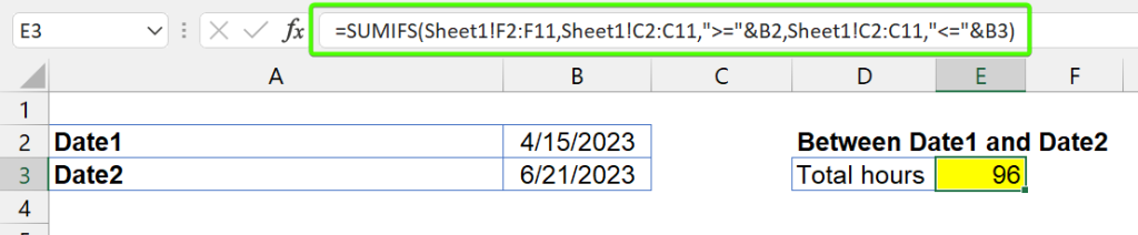
Notice that, in the above case, you just need to add the sheet name followed by an exclamation point (Sheet1!) for the range of cells you want to sum and the range that contains the criteria.
Excel SUMIF date in a specific month
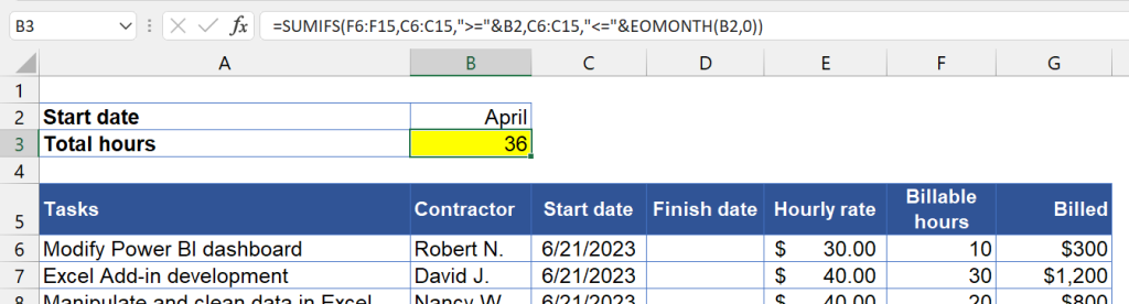
The following example shows how to get the total hours for tasks that started in April 2023.

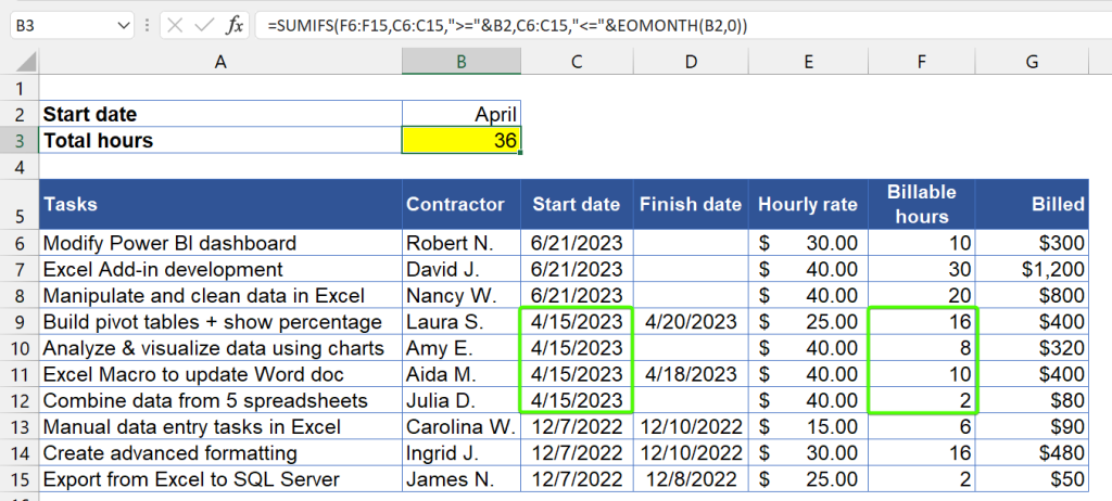
Here’s the formula in B3, which uses a SUMIFS function with two criteria — start date is >= first day of April 2023 AND end date is <= last day of April 2023:
=SUMIFS(F6:F15,C6:C15,">="&B2,C6:C15,"<="&EOMONTH(B2,0))
To get the above formula, you can follow the steps below:
Step 1: Type the first date of April 2023 in B2.

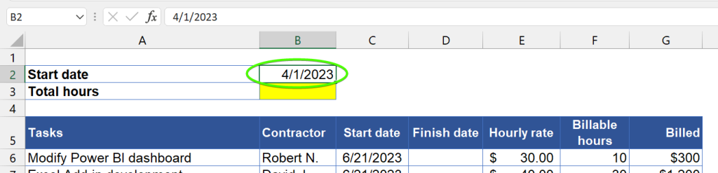
Step 2: Right-click on the cell and select Format cells => Custom and specify mmmm in the Type. This will change the format of B2 to display the name of the month.

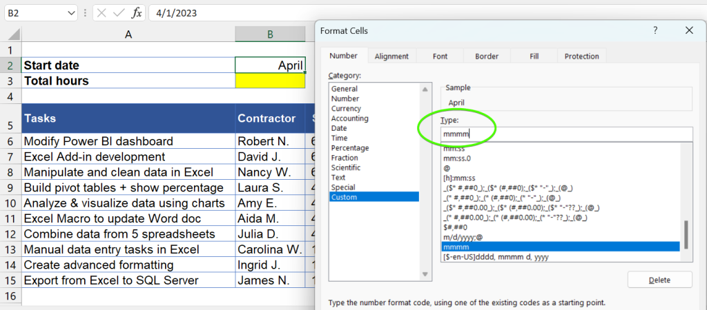
Step 3: Write the following formula in B3, then press Enter. Note: The EOMONTH function helps you to find the last day of the month.
=SUMIFS(F6:F15,C6:C15,">="&B2,C6:C15,"<="&EOMONTH(B2,0))

Excel SUMIF date in a specific year
The following example shows how to calculate the total hours for all the tasks that started in 2023:

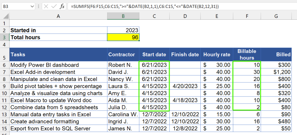
Formula in B3:
=SUMIFS(F6:F15,C6:C15,">="&DATE(B2,1,1),C6:C15,"<="&DATE(B2,12,31))
The above formula uses SUMIFS with these two criteria: start date is >= January 1, 2023 AND end date is <= December 31, 2023.
Excel SUMIF date criteria in multiple columns
The following example shows how to get the total hours for all the completed tasks that started on April 15, 2023.

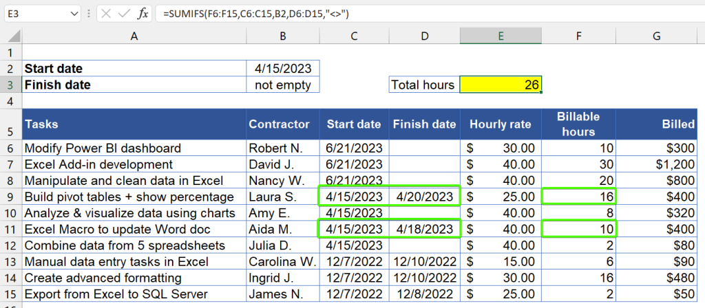
Formula in E3:
=SUMIFS(F6:F15,C6:C15,B2,D6:D15,"<>")
Notice that in this case, we use SUMIFS with criteria in two different columns: Start date and Finish date. The first criterion is for the start dates that are equal to April 15, 2023, and the second criterion is for the finish dates that are not empty.
How to automate data import to Excel
Are you still manually getting your data to Excel before summing it with SUMIF and SUMIFS? If yes, now you don’t have to copy and paste anymore! To save you time and reduce the likelihood of errors, you can automate this process with Coupler.io.
Use the form below to see how it works: choose your data source and click Proceed. You can sign up with your Microsoft account for free. Next, select your metrics, report period, and refresh schedule. In a few steps, you’ll have your data imported and updated automatically.
