The VLOOKUP function looks up only one value. And what if you want to return a result that matches two values within a range? Check out the following workaround.
How to VLOOKUP for two values
We imported a dataset from Google Sheets to Excel using Coupler.io, a solution for automatic data exports from multiple apps and sources. Read more about Microsoft Excel integrations for data export on a schedule.
Our purpose is to look up a car value for a user with the name “Mella“, and the Excel VLOOKUP function can do the job easily. The issue is that we have multiple users with the name “Mella“.
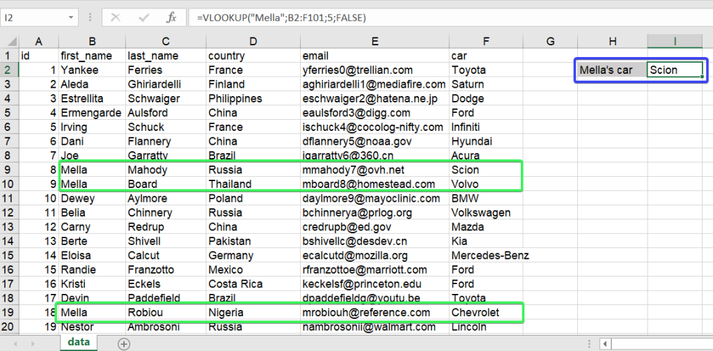
So, we need to narrow down our lookup using two criteria:
- Name – “Mella“
- Country – “Nigeria“
You can’t specify two lookup values in a VLOOKUP formula, so we’ll need to use a workaround, which consists of two steps:
- Step1: Create a separate column where we will create unique lookup_values by merging our two lookup criteria – name and country – for example “MellaThailand“, “MellaNigeria“, etc.
- Step2: Look up the range using the unique strings as the lookup_value to return a matching value.
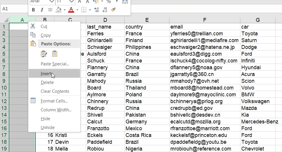
Step1: Create a column with unique lookup_values made of two lookup criteria
- Insert a column to the left of your dataset like this:
- Select the entire column, insert the following formula to the formula bar and press Ctrl+Shift+Enter for Windows (Command+Return for Mac) – This will apply an array formula in Excel:
=C1:C100&E1:E1000

This formula will merge two values from columns C and E in the specified array.
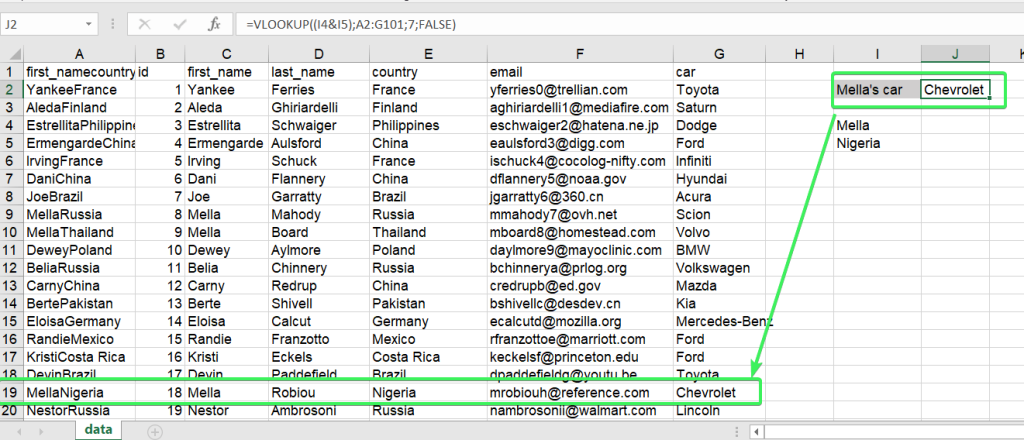
Step2: VLOOKUP formula for two values
Now we can insert a VLOOKUP formula, which will contain two lookup_values merged into one:
=VLOOKUP((I4&I5),A2:G101,7,FALSE)
(I4&I5)– a lookup value based on the formula, which merges values from cells I4 (Mella) and I5 (Nigeria).A2:G101– the range to look up7– the column to return the matching values from
You can apply the same logic for using more than two criteria as a lookup value.