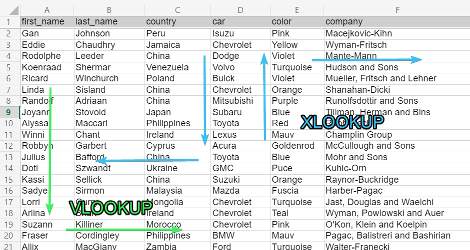
Excel XLOOKUP - The Advanced LOOKUP Function

VLOOKUP in Excel allows you to search for a match for a specified lookup value to the right of it. If you need to make a reverse lookup – to the left – the XLOOKUP function in Excel will do the job.

However, it is not the only direction this function can cover. Read on to explore further details.

XLOOKUP in Excel – VLOOKUP, HLOOKUP and LOOKUP in one function

The first thing you should know about the XLOOKUP function is that it is only available in Microsoft Excel Online and Microsoft 365.

XLOOKUP is the function that provides a two-way lookup:

Lookup to the left or right or both (alternative to the VLOOKUP function)

Lookup from top to bottom or from bottom to top (alternative to the HLOOKUP function)

Lookup exact matches or partial matches using wildcards

Excel XLOOKUP function syntax

=XLOOKUP("lookup_value", lookup_array, return_array, "[if_not_found]", [match_mode], [search_mode])

"lookup_value" – the value to look up. The string as a lookup value should be enclosed in quotes; a cell reference as a lookup value should not be enclosed in quotes.
lookup_array – the array to search the lookup value.
return_array – the array to return the matching value from.
[if_not_found] – the text to return if the lookup value has not been found. Optional parameter.
[match_mode] – the match mode for the lookup. Optional parameter.
[search_mode] – the search mode for the lookup. Optional parameter.

Excel XLOOKUP formula example

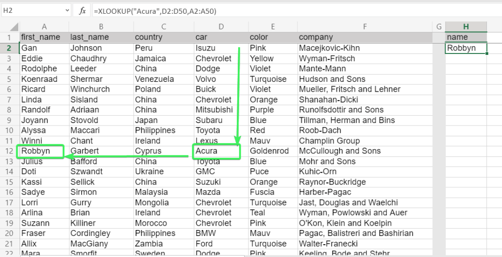
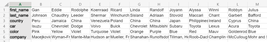
Let’s check out how XLOOKUP works in the example of a simple lookup without optional arguments. We have a dataset that we loaded to Excel using Coupler.io, a reporting automation solution.

The XLOOKUP function will help us find the name of the owner of an Acura in the first columns. Here is the formula:

=XLOOKUP("Acura",D2:D50,A2:A50)

"Acura" – the lookup value
D2:D50 – the array to search for the lookup value
A2:A50 – the array to return the matching value from

XLOOKUP examples with optional arguments

Now let’s look at more advanced examples of Excel formulas with this advanced lookup function using optional parameters.

Excel XLOOKUP with match_mode argument

The [match_mode] is the fifth parameter in the XLOOKUP formula. It is denoted as a numeral from -1 to 2 which correspond to the following match types:

0 – An exact match (default).
-1 – The next smallest item if no exact match.
1 – The next largest item if no exact match.
2 – A wildcard match.

With a wildcard match, you need to use wildcards (*, ?, or ~) when specifying a lookup value. They have the following meanings:

* – To replace multiple characters.
? – To replace any single character.
~ – Used with asterisk (*) and question mark (?), as well as tilde (~) to denote their literal meaning.

Wildcards only work with textual values

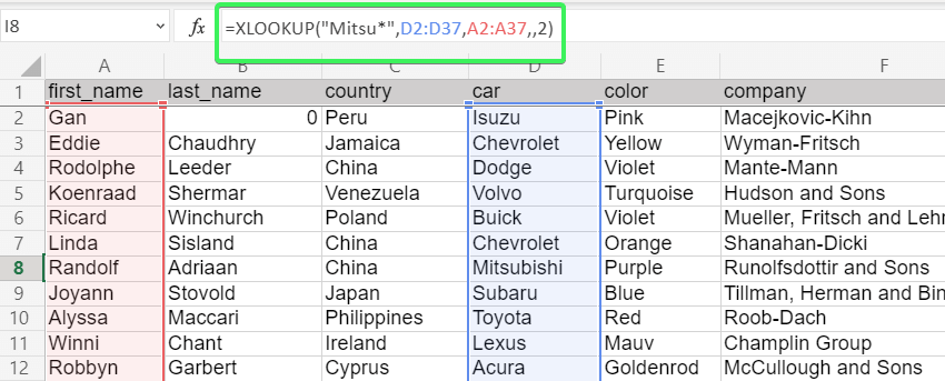
As an example, let’s lookup an approximate match – find the name of the owner of the car with the brand name starting with “M”. Here is the XLOOKUP formula:

=XLOOKUP("M*",D2:D50,A2:A50,,2)

"M*" – the lookup value for a text that starts with M
D2:D50 – the array to search for the lookup value
A2:A50 – the array to return the matching value from
2 – wildcard match mode

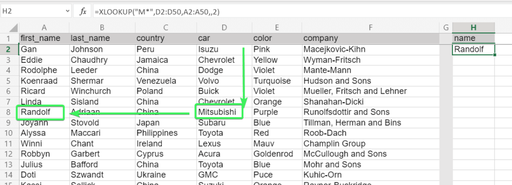
The formula returned “Randolf” who drives a Mitsubishi and is the first match from the top. Now, what if you want to look up the first match from the bottom? In this case, choose a respective search mode.

Excel XLOOKUP search mode

The [search_mode] is the sixth parameter in the XLOOKUP formula. It is denoted as a numeral from -2 to 2 with 0 excluded:

1 – Lookup from the top (default).
-1 – Lookup from the bottom.
2 – Fast search based on a binary search algorithm for the lookup array sorted in ascending order. If not sorted, invalid results will be returned.
-2 – Fast search based on a binary search algorithm for the lookup array sorted in descending order. If not sorted, invalid results will be returned.

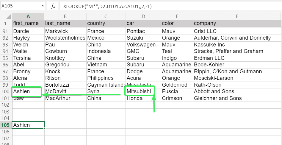
As an example, let’s find the name of the owner of the car with the brand name starting with “M“. This time, the lookup will start from the bottom. Here is the XLOOKUP formula:

=XLOOKUP("M*",D2:D101,A2:A101,,2,-1)

"M*" – the lookup value for a text that starts with M
D2:D101 – the array to search for the lookup value
A2:A101 – the array to return the matching value from
2 – wildcard match mode
-1 – search mode from the bottom

How to use XLOOKUP with multiple criteria

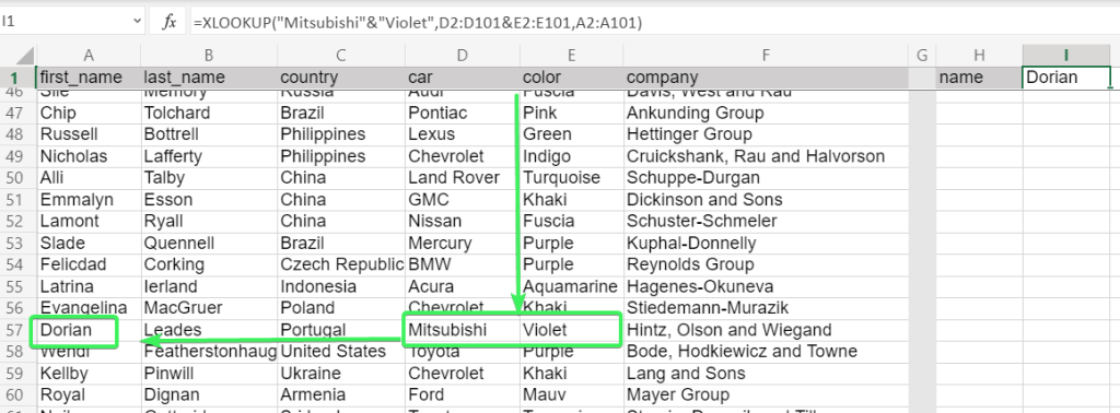
The more criteria you have, the more accurate the xmatch is, right? For example, in our data set, there are multiple Mitsubishi owners and we need to look up the one who drives a violet Mitsubishi. So, we have two criteria (lookup values) to search for a match. XLOOKUP allows you to do this with the following syntax:

=XLOOKUP("lookup_value1"&"lookup_value2"&...,lookup_array1&lookup_array2&..., return_array, "[if_not_found]", [match_mode], [search_mode])

The only difference in syntax between XLOOKUP with one criterion and XLOOKUP with multiple criteria is that you need to add the required lookup values and lookup arrays using the ampersand (&).

Here is an example of the XLOOKUP formula with multiple criteria:

=XLOOKUP("Mitsubishi"&"Violet",D2:D101&E2:E101,A2:A101)

Is there any XLOOKUP vs. INDEX MATCH speed difference?

In our Excel VLOOKUP tutorial, we mentioned the combination of the INDEX and MATCH functions to implement a reverse vertical lookup. Basically, this is a workaround for those Excel users who do not have XLOOKUP. Which option is more efficient?

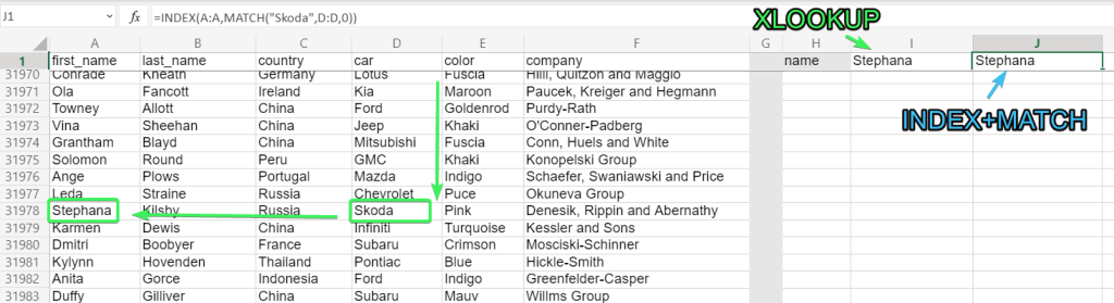
We tested both on a dataset with 192,000 cells, however, we did not notice any difference in speed. Here are the formulas we used:

XLOOKUP:

=XLOOKUP("Skoda",D:D,A:A)

INDEX+MATCH:

=INDEX(A:A,MATCH("Skoda",D:D,0))

For larger datasets, it is likely that XLOOKUP will be more efficient if you use a binary search mode. The syntax of XLOOKUP is also much simpler compared to INDEX+MATCH. However, if you don’t have access to XLOOKUP, then INDEX and MATCH should definitely be your next choice.

What does XLOOKUP for a horizontal lookup look like?

As a final word, let’s show how you can use XLOOKUP to look up horizontally, not just vertically. We have transposed our dataset in our worksheet, so now it looks as follows:

And here is the XLOOKUP formula to search horizontally for a Toyota owner:

=XLOOKUP("Toyota",B4:CW4,B1:CW1)

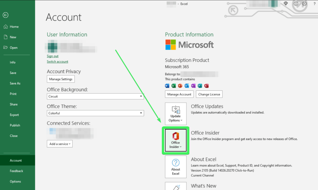
How to get XLOOKUP function if you don’t have it in your workbook

Users of Microsoft 365 already have access to XLOOKUP without taking any additional actions. For some older versions of Excel, such as Home, Personal, or University, you need to join the Office Insider program as follows:

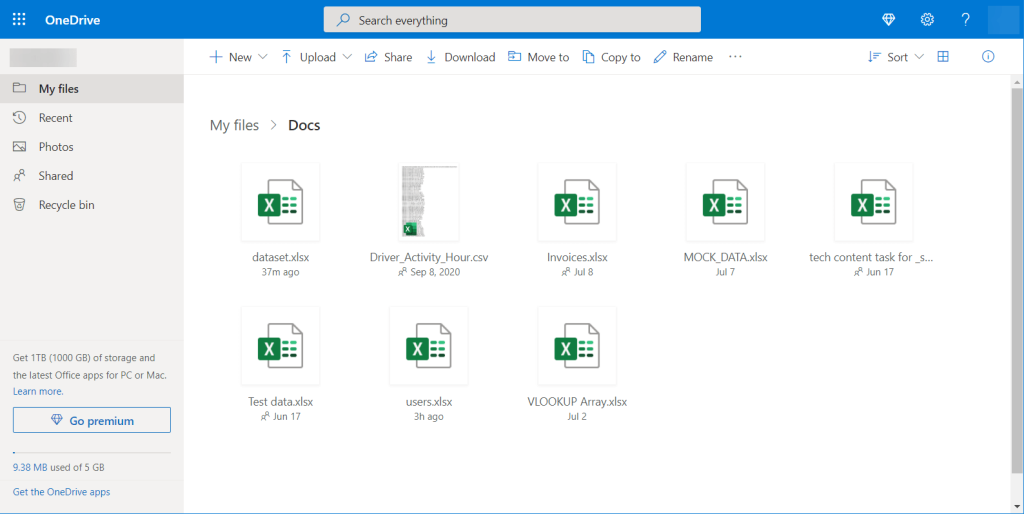
XLOOKUP cannot be implemented in Excel 2019 or earlier versions. However, you can use Excel Online instead. All you need to do is drop your Excel files in the OneDrive folder on your PC and sign into OneDrive on the web. Here is how your OneDrive folder will look in your internet browser:

Now you can open your files in Excel Online and enjoy the power of XLOOKUP.

Automate data import from cloud sources to Excel

In this Excel tutorial, we mentioned Coupler.io as a solution for importing data to Excel. It lets you connect 60+ cloud data sources and automate data exports on a schedule to your workbook.

You can try it yourself for free right away – select the needed source application in the form below and click Proceed.

You’ll be offered to create a Coupler.io account for free.

After that configure the connection of your source application and choose the Excel workbook and worksheet for your data.

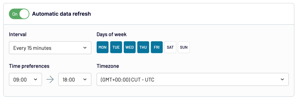
As the final step, set up a schedule for automatic data refresh to always access the recent data from your source in Excel.

In addition to Excel, Coupler.io supports other destination apps including Power BI, Google Sheets, Looker Studio, and more.

That’s it! Master your Excel skills and good luck with your data!

Zakhar Yung

A content manager at Coupler.io whose key responsibility is to ensure that the readers love our content on the blog. With 5 years of experience as a wordsmith in SaaS, I know how to make texts resonate with readers' queries??