Coupler.io Blog

How to Use IMPORTRANGE in Google Sheets to Import Data Across Spreadsheets

Zakhar Yung

1 year ago

Importrange tutorial

To import a data range from another spreadsheet (Google Sheets document), there is a Google Sheets function – IMPORTRANGE. Let’s check out how it works and discover the IMPORTRANGE alternative, which lets you automate data import across spreadsheets.

Some users may prefer watching to reading. In this case, check out this step-by-step IMPORTRANGE function tutorial for Google Sheets by Coupler.io Academy.

Understanding IMPORTRANGE Google Sheets

IMPORTRANGE allows you to import a data range from one spreadsheet to another. It’s a pure Google Sheets function – i.e. there is no Excel IMPORTRANGE.

Do not confuse IMPORTRANGE with IMPORTDATA, which imports data from online published CSV or TSV files. Check out our dedicated blog post about Google Sheets IMPORTDATA Function.

IMPORTRANGE Google Sheets syntax

=IMPORTRANGE("spreadsheet","range_string")

spreadsheet – insert the URL or ID of the spreadsheet to import data from.
range_string – insert a string that specifies the data range to import. The string should include the name of the sheet and the range of cells.

Google Sheets IMPORTRANGE formula example

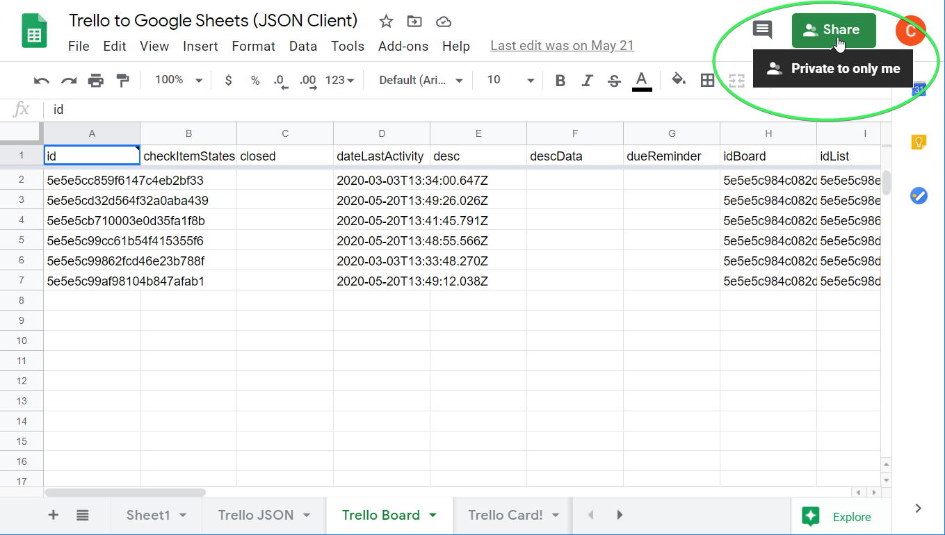
We have a spreadsheet with the data imported from Trello. Let’s pull columns A to E from it. Use the formula with the spreadsheet URL:

=importrange("https://docs.google.com/spreadsheets/d/1jUPrXMmsZwJNnWcxm-pRVz1xBY-TEoVGsq5c2jHunvI/edit#gid=590318270","Trello Board!A:E")

or with the spreadsheet ID:

=importrange("1jUPrXMmsZwJNnWcxm-pRVz1xBY-TEoVGsq5c2jHunvI","Trello Board!A:E")

IMPORTRANGE Allow Access to the spreadsheet in Google Sheets

When you import a range from an unshared spreadsheet, IMPORTRANGE will require you to connect the source and the target spreadsheets.

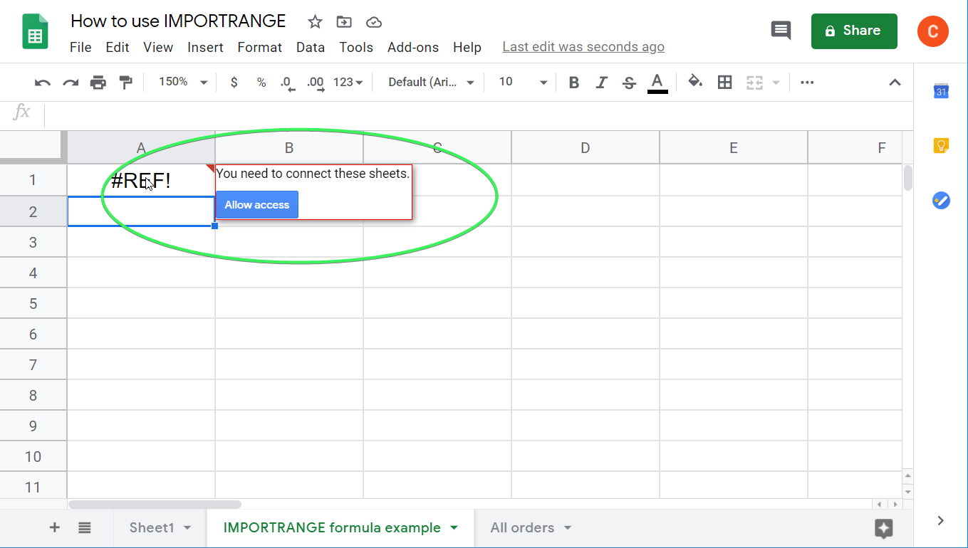
Click Allow access, and IMPORTRANGE will then work. You’ll have to do this only once, at the first data import.

Note: When you allow access for IMPORTRANGE, you do NOT change the SHARE status of your spreadsheet.

Meanwhile, you can’t revoke the connection if both the source and the target spreadsheets belong to the same user.

Google Sheets IMPORTRANGE drawbacks

Poor import performance if multiple IMPORTRANGE formulas are used. The more IMPORTRANGE formulas your spreadsheet has, the more time it will require to process requests. At some point, it can even stop working completely.
Data loads only when the spreadsheet is open. The imported data may not be available until you open the spreadsheet with the IMPORTRANGE formula. This is troublesome if the data in the spreadsheet is synchronized with a third-party app or tool.
Limited functionality. With IMPORTRANGE, you can’t import the entire sheet; you have to specify a cell range; you can’t schedule data import; you can’t import a consolidation of sheets from a spreadsheet, etc.

If you’ve faced any of the issues above, you might need an IMPORTRANGE Google Sheets alternative.

IMPORTRANGE Google Sheets alternative to automate data import on a schedule

The Google Sheets integration by Coupler.io lacks the IMPORTRANGE drawbacks mentioned above. It’s an option in Google Sheets to reference another sheet and import data across Google Sheets. Moreover, it allows you to preview and transform the imported data on the go before loading it to the target spreadsheet. This includes column management, data filtering, sorting, data blending, and more.

It takes three simple steps to connect one spreadsheet with another.

1. Collect data from the source spreadsheet

Click Proceed in the form below. You’ll be offered to get started with Coupler.io for free with no credit card required.

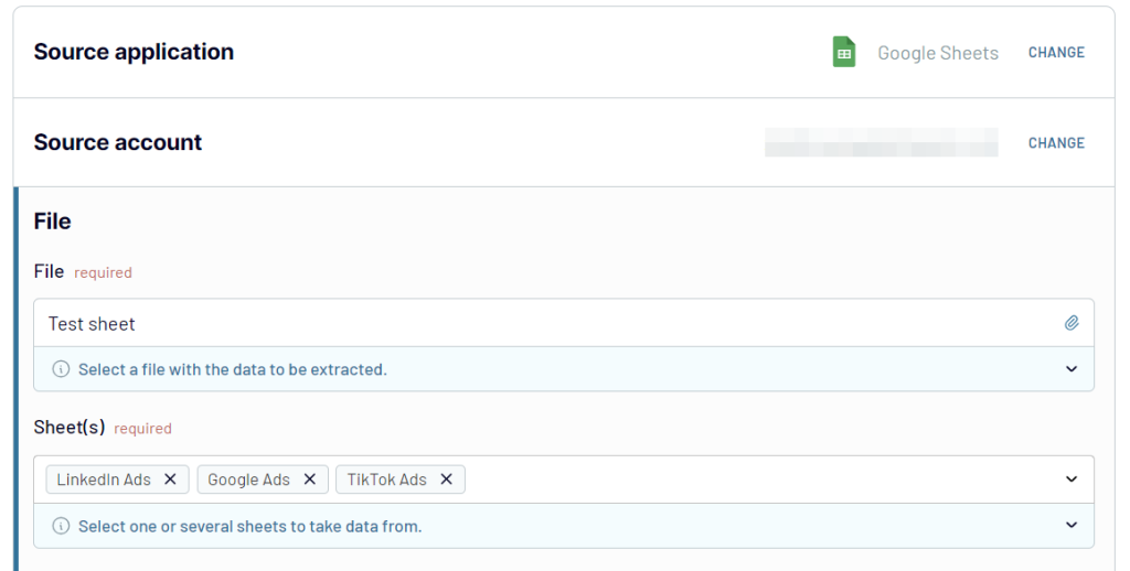
Connect your Google account, then select a Google Sheets file on your Google Drive to transfer data from. Select one or several sheets to export data. The latter option lets you merge multiple sheets into one master view.

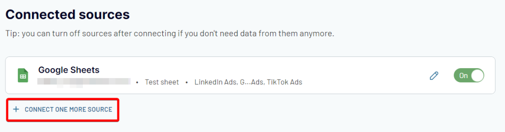
With Coupler.io, you can import data from multiple sheets and multiple Google Sheets files. For the latter, you need to click +Connect one more source and configure the connection in a similar way as above.

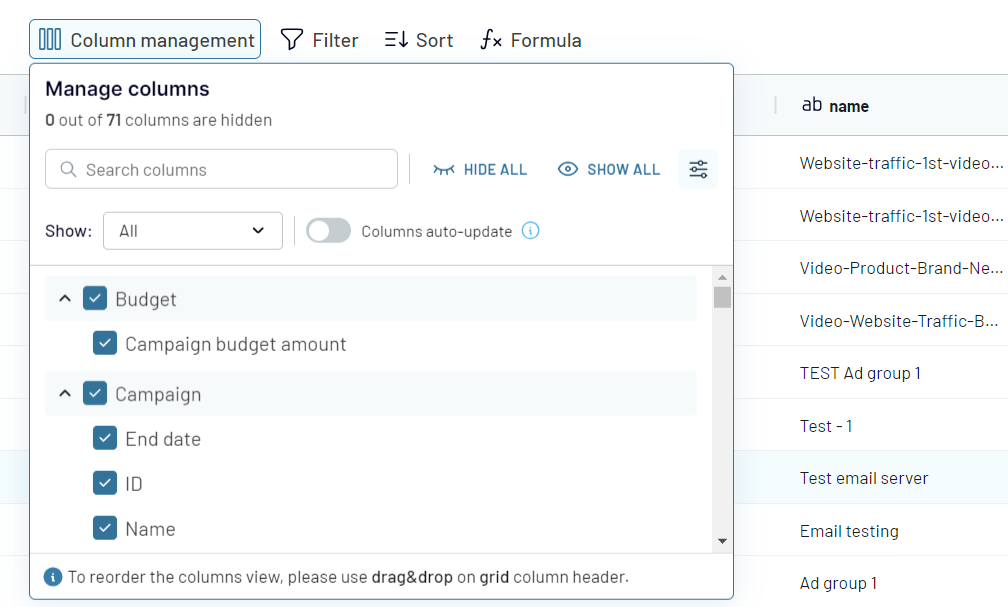
2. Preview and transform data

Now you can preview the imported data and transform it:

Hide columns you won’t need
Edit or rearrange columns
Add new columns
Filter and sort records
Join data if you’ve connected multiple spreadsheets.

3. Load data and schedule refresh

Connect your Google account and choose a Google Sheets file on your Google Drive to transfer data to. Type a name to create a new sheet or pick an existing one.

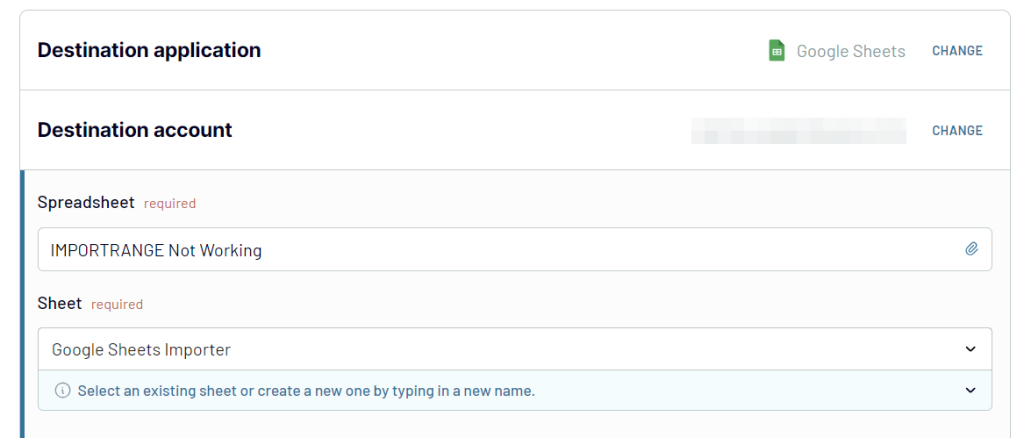
Optionally, you can change the first cell where to import your data range, change the import mode, and use other features. To keep your spreadsheets linked, automate data imports. For this, toggle on the Automatic data refresh and set up a schedule.

You can also use Coupler.io as a Google Sheets add-on to have faster access to the tool in your Google Sheets. For this install it from the Google Workspace Marketplace and set it up as we described above.

Try Coupler.io for free

IMPORTRANGE Google Sheets how-to guide

This will cover how to use IMPORTRANGE in practice, and various tasks that you can carry out with this Google Sheets function.

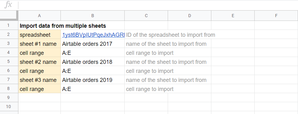
How to import data from multiple sheets with IMPORTRANGE in Google Sheets

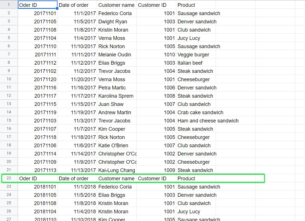
We need to import the same data range (A:E) from three sheets (Airtable orders 2017, Airtable orders 2018, and Airtable orders 2019) of one spreadsheet.

You can import data with IMPORTRANGE with the following options:

Import and merge data vertically

If you’re importing a limited data range like A1:E21, you can use an array (curly brackets) and IMPORTRANGE formulas separated with semicolons. For example:

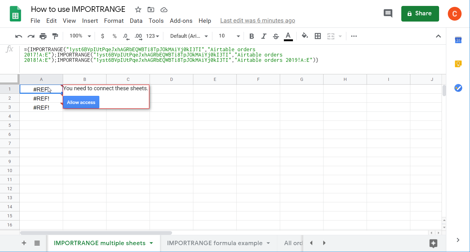
={IMPORTRANGE("1yst6BVpIUtPqeJxhAGRbEQWBTi8TpJOkMAiYj0kI3TI","Airtable orders 2017!A1:E21");
IMPORTRANGE("1yst6BVpIUtPqeJxhAGRbEQWBTi8TpJOkMAiYj0kI3TI","Airtable orders 2018!A1:E21");
IMPORTRANGE("1yst6BVpIUtPqeJxhAGRbEQWBTi8TpJOkMAiYj0kI3TI","Airtable orders 2019!A1:E21")}

Click Allow access to connect the sheets.

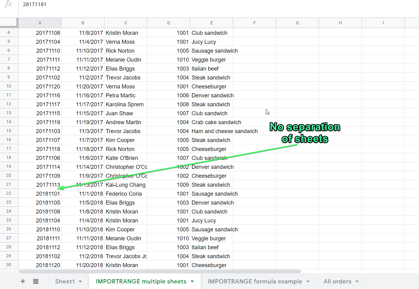
The data will be imported and merged vertically. However, to import and merge an unlimited data range (A1:E), you’ll need to nest IMPORTRANGE with FILTER and LEN as follows:

={FILTER(IMPORTRANGE("{spreadsheet-ID}", "{sheet#1-name}!{sheet#1-range}"),LEN(IMPORTRANGE("{spreadsheet-ID}", "{sheet#1-name}!{sheet#1-first-column})>0);
FILTER(IMPORTRANGE("{spreadsheet-ID}", "{sheet#2-name}!{sheet#2-range}"),LEN(IMPORTRANGE("{spreadsheet-ID}", "{sheet#2-name}!{sheet#2-first-column})>0);...}

{spreadsheet-ID} – the ID or URL of the Google Sheets document, you’re importing data from
{sheet#1-name} – the name of the first sheet
{sheet#1-name} – the name of the second sheet
{sheet#2-range} – the data range from the first sheet including the title row.
{sheet#2-range} – the data range from the second sheet without the title row.
{sheet#1-first-column} – the first column of the data range from the first sheet.
{sheet#2-first-column} – the first column (without the title row) of the data range from the second sheet.

In our case, the formula will look like this:

={FILTER(IMPORTRANGE("1yst6BVpIUtPqeJxhAGRbEQWBTi8TpJOkMAiYj0kI3TI","Airtable orders 2017!A1:E"),LEN(IMPORTRANGE("1yst6BVpIUtPqeJxhAGRbEQWBTi8TpJOkMAiYj0kI3TI","Airtable orders 2017!A1:A")));
FILTER(IMPORTRANGE("1yst6BVpIUtPqeJxhAGRbEQWBTi8TpJOkMAiYj0kI3TI","Airtable orders 2018!A1:E"),LEN(IMPORTRANGE("1yst6BVpIUtPqeJxhAGRbEQWBTi8TpJOkMAiYj0kI3TI","Airtable orders 2018!A1:A")));
FILTER(IMPORTRANGE("1yst6BVpIUtPqeJxhAGRbEQWBTi8TpJOkMAiYj0kI3TI","Airtable orders 2019!A1:E"),LEN(IMPORTRANGE("1yst6BVpIUtPqeJxhAGRbEQWBTi8TpJOkMAiYj0kI3TI","Airtable orders 2019!A1:A")))}

In our formula, we used the same data range for all sheets including the first rows from each sheet.

If you don’t need this, replace A1:E with A2:E for the second and the third sheets to merge:

={FILTER(IMPORTRANGE("1yst6BVpIUtPqeJxhAGRbEQWBTi8TpJOkMAiYj0kI3TI","Airtable orders 2017!A1:E"),LEN(IMPORTRANGE("1yst6BVpIUtPqeJxhAGRbEQWBTi8TpJOkMAiYj0kI3TI","Airtable orders 2017!A1:A")));
FILTER(IMPORTRANGE("1yst6BVpIUtPqeJxhAGRbEQWBTi8TpJOkMAiYj0kI3TI","Airtable orders 2018!A2:E"),LEN(IMPORTRANGE("1yst6BVpIUtPqeJxhAGRbEQWBTi8TpJOkMAiYj0kI3TI","Airtable orders 2018!A1:A")));
FILTER(IMPORTRANGE("1yst6BVpIUtPqeJxhAGRbEQWBTi8TpJOkMAiYj0kI3TI","Airtable orders 2019!A2:E"),LEN(IMPORTRANGE("1yst6BVpIUtPqeJxhAGRbEQWBTi8TpJOkMAiYj0kI3TI","Airtable orders 2019!A1:A")))}

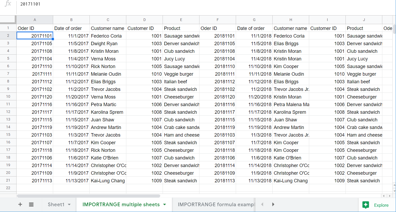
Import and merge data horizontally

You can import and append data horizontally with IMPORTRANGE only if the data range to fetch in each sheet is the same. In order to do this correctly, use an array (curly brackets) and several IMPORTRANGE formulas separated with commas:

={IMPORTRANGE("1yst6BVpIUtPqeJxhAGRbEQWBTi8TpJOkMAiYj0kI3TI","Airtable orders 2017!A:E"),
IMPORTRANGE("1yst6BVpIUtPqeJxhAGRbEQWBTi8TpJOkMAiYj0kI3TI","Airtable orders 2018!A:E"),
IMPORTRANGE("1yst6BVpIUtPqeJxhAGRbEQWBTi8TpJOkMAiYj0kI3TI","Airtable orders 2019!A:E")}

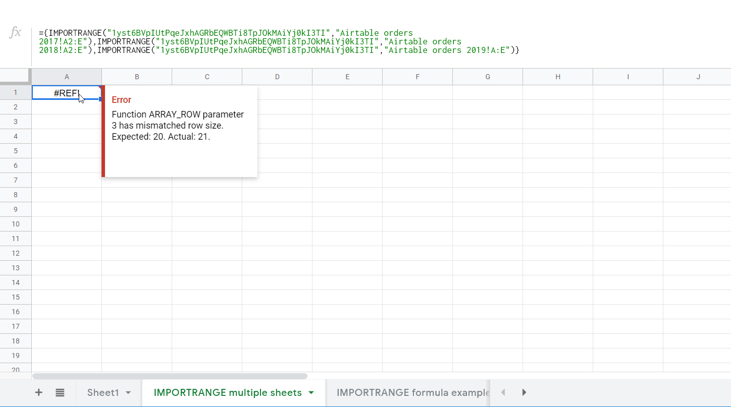
If you try to import different data ranges, the IMPORTRANGE formula will return an Error: Function ARRAY_ROW parameter 3 has mismatched row size. Expected: 20. Actual: 21.

={IMPORTRANGE("1yst6BVpIUtPqeJxhAGRbEQWBTi8TpJOkMAiYj0kI3TI","Airtable orders 2017!A2:E"),
IMPORTRANGE("1yst6BVpIUtPqeJxhAGRbEQWBTi8TpJOkMAiYj0kI3TI","Airtable orders 2018!A2:E"),
IMPORTRANGE("1yst6BVpIUtPqeJxhAGRbEQWBTi8TpJOkMAiYj0kI3TI","Airtable orders 2019!A:E")}

For more on this, read our blog post Why IMPORTRANGE Is Not Working: Errors and Fixes.

Import data from multiple sheets with the IMPORTRANGE alternative in Google Sheets

With the Google Sheets integration by Coupler.io, you can import data from multiple sheets more easily. You need to specify the following parameters:

the names of the sheets to merge
the data range

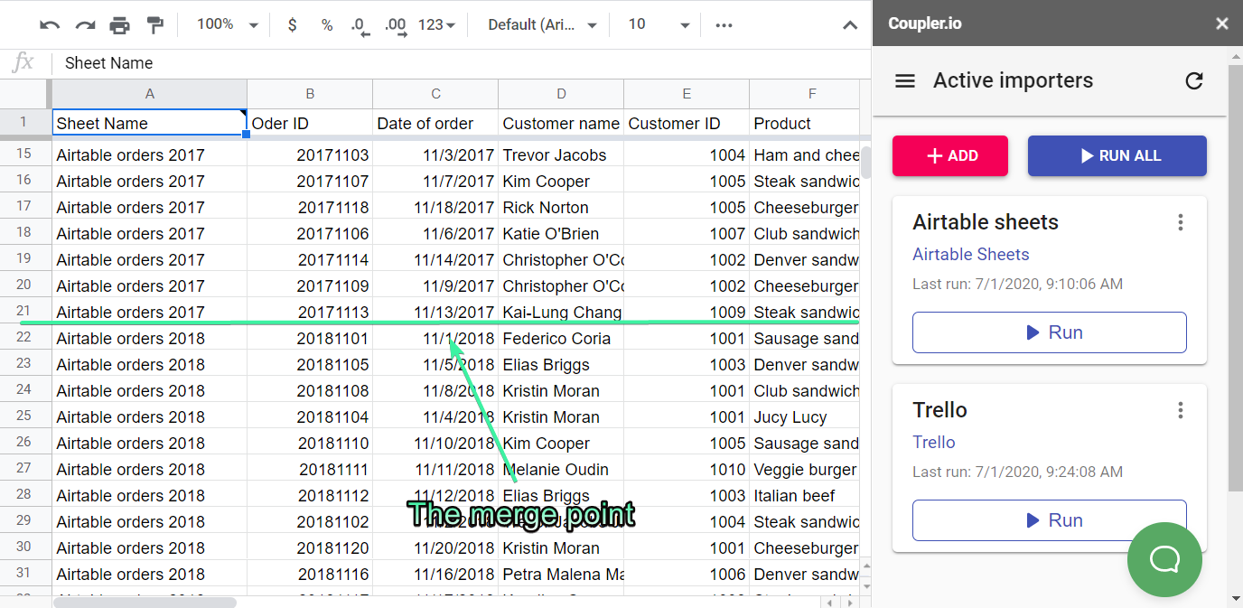
Once you run the integration, it will import and merge data vertically. The Google Sheets integration adds a Sheet Name column, so you could differentiate where the data came from. It also automatically skips the column headers from the appended sheets if they are identical to the column headers of the first sheet.

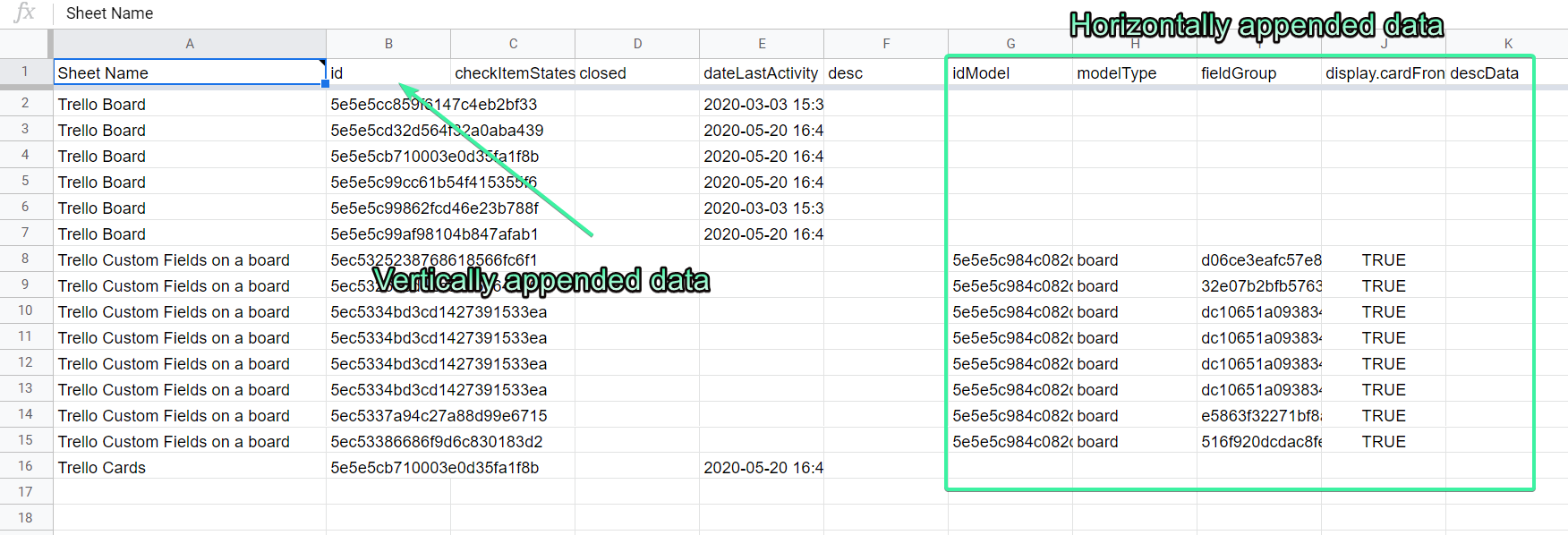
If the specified sheets have different column headers, the importer will merge vertically only the identical ones, and the rest will be appended horizontally to the right. Here is how it will look:

How to import data from multiple spreadsheets with IMPORTRANGE Google Sheets

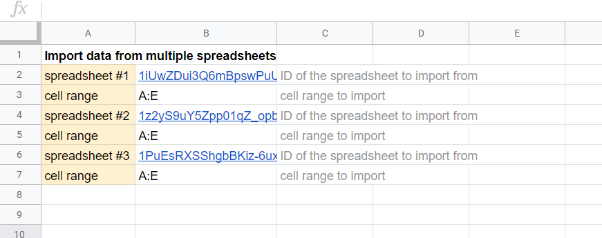
We need to import the same data range (A:E) from three separate spreadsheets.

Import and merge data vertically

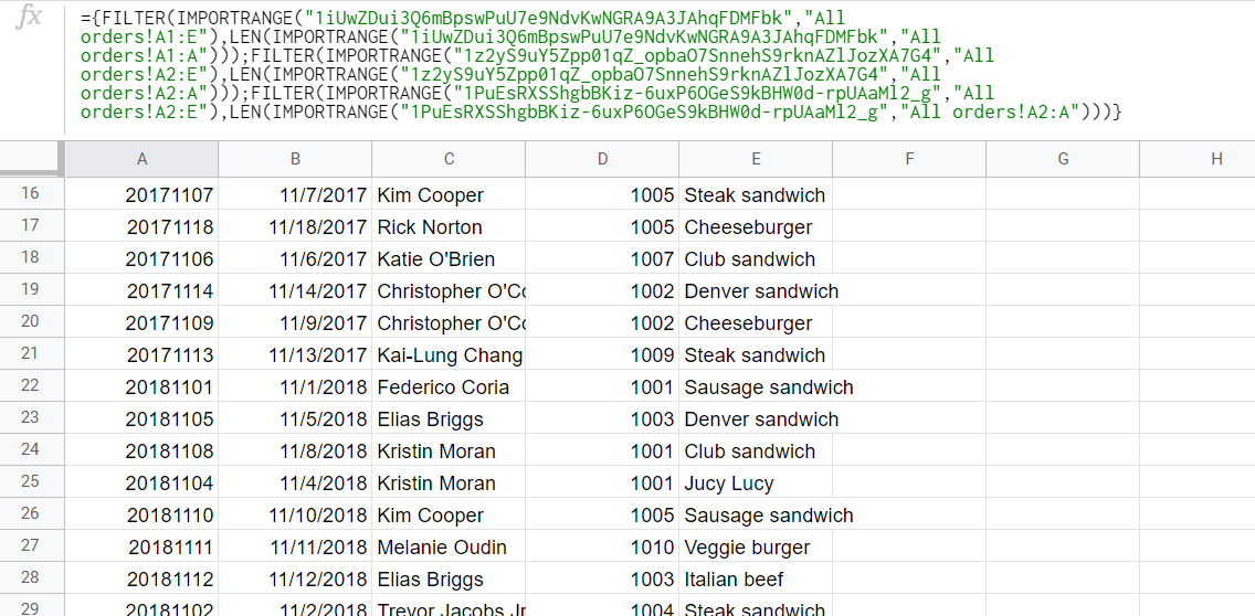
Use an array (curly brackets) and IMPORTRANGE formulas nested with FILTER and LEN:

={FILTER(IMPORTRANGE("1iUwZDui3Q6mBpswPuU7e9NdvKwNGRA9A3JAhqFDMFbk","All orders!A1:E"),LEN(IMPORTRANGE("1iUwZDui3Q6mBpswPuU7e9NdvKwNGRA9A3JAhqFDMFbk","All orders!A1:A"));
FILTER(IMPORTRANGE("1z2yS9uY5Zpp01qZ_opbaO7SnnehS9rknAZlJozXA7G4","All orders!A2:E"),LEN(IMPORTRANGE("1z2yS9uY5Zpp01qZ_opbaO7SnnehS9rknAZlJozXA7G4","All orders!A2:A"));
FILTER(IMPORTRANGE("1PuEsRXSShgbBKiz-6uxP6OGeS9kBHW0d-rpUAaMl2_g","All orders!A2:E"),LEN(IMPORTRANGE("1PuEsRXSShgbBKiz-6uxP6OGeS9kBHW0d-rpUAaMl2_g","All orders!A2:A"))}

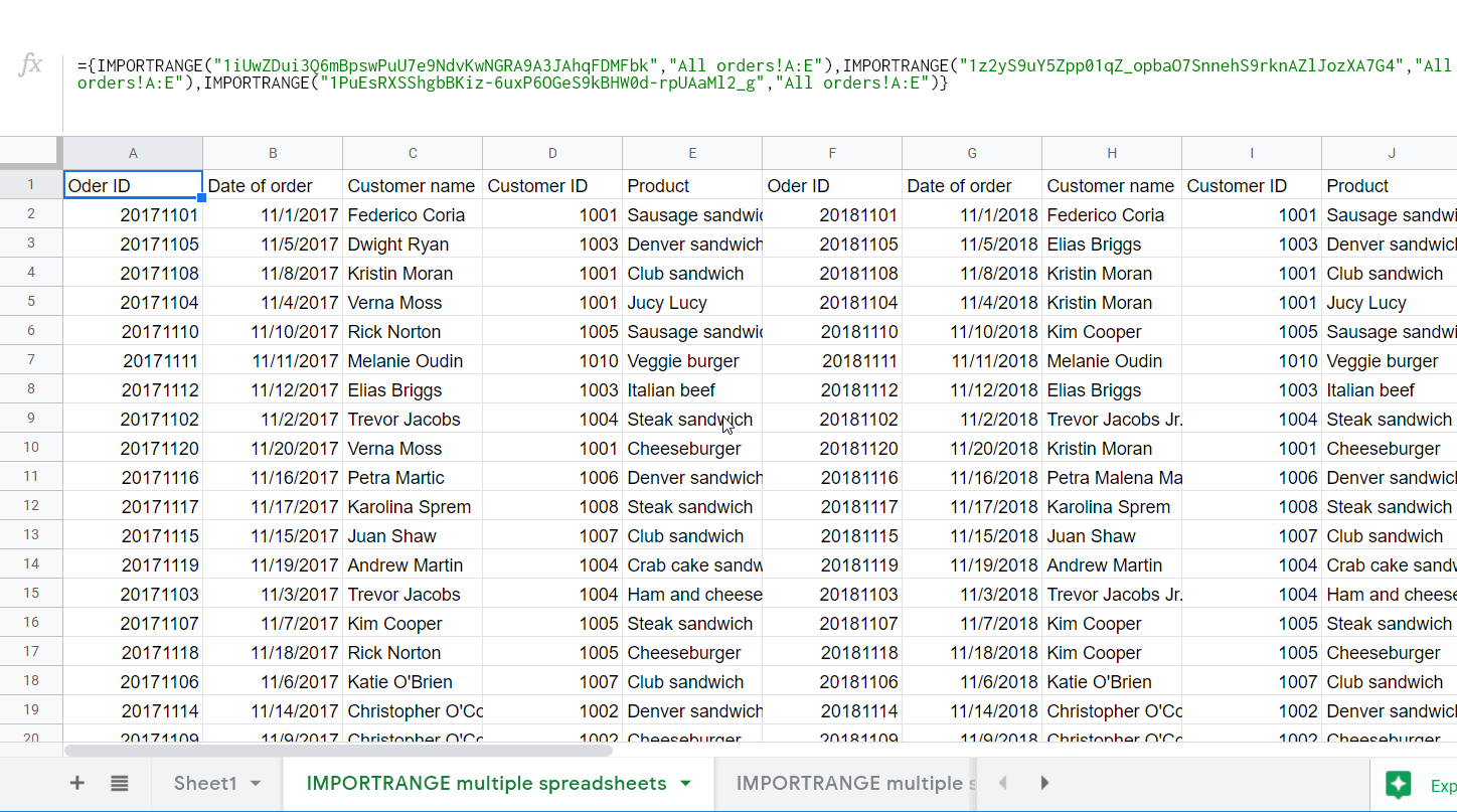
Import and merge data horizontally

You can import and append data horizontally with IMPORTRANGE only if the data range to fetch in each sheet is the same. To do this in the correct way, use an array (curly brackets) and several IMPORTRANGE formulas separated with commas:

={IMPORTRANGE("1iUwZDui3Q6mBpswPuU7e9NdvKwNGRA9A3JAhqFDMFbk","All orders!A:E"),
IMPORTRANGE("1z2yS9uY5Zpp01qZ_opbaO7SnnehS9rknAZlJozXA7G4","All orders!A:E"),
IMPORTRANGE("1PuEsRXSShgbBKiz-6uxP6OGeS9kBHW0d-rpUAaMl2_g","All orders!A:E")}

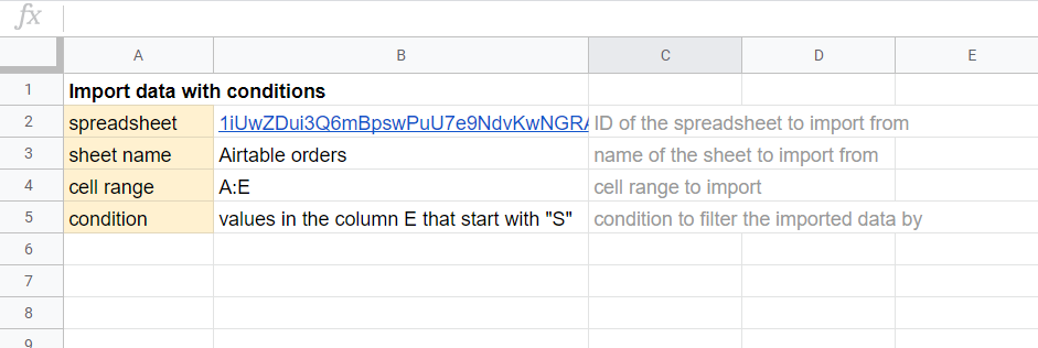
How to IMPORTRANGE with conditions in Google Sheets?

If you combine IMPORTRANGE with the QUERY function, you can import data across spreadsheets according to different conditions such as:

Import a specific range of data
Cut off unnecessary rows of the imported data
Change names of the imported columns
Format values in the imported columns
Import the filtered data
Sort the imported data
Perform arithmetic, aggregation, and scalar operations on the imported data

For more on Google Sheets QUERY Function, read our dedicated blog post.
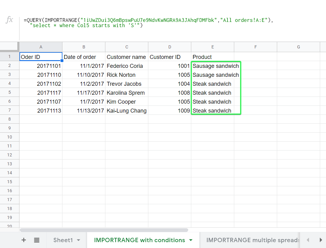
Let’s check out how it works on a simple example: We’ll import a data range A:E from a spreadsheet, and filter the imported data on the values in column E that start with the letter “S“.

Here is how the formula will look:

=QUERY(IMPORTRANGE("1iUwZDui3Q6mBpswPuU7e9NdvKwNGRA9A3JAhqFDMFbk","All orders!A:E"),
  "select * where Col5 starts with 'S'")

How to hide formulas with IMPORTRANGE Google Sheets?

Let’s say you have a spreadsheet that some stakeholders can view. This spreadsheet contains specific formulas you’re not willing to disclose. How can you let the stakeholders see the values, and hide the formulas at the same time?

If this is what you need, IMPORTRANGE can offer you a workaround to hide formulas. The idea is to create two Google Sheets documents:

In the first one, you will store formulas.
In the second one, you will import the values from the first spreadsheet using IMPORTRANGE.

For example, the original spreadsheet with our formulas is called “Formulas to hide”. It contains three formulas: COUNTIF, FILTER, and SUMIF.

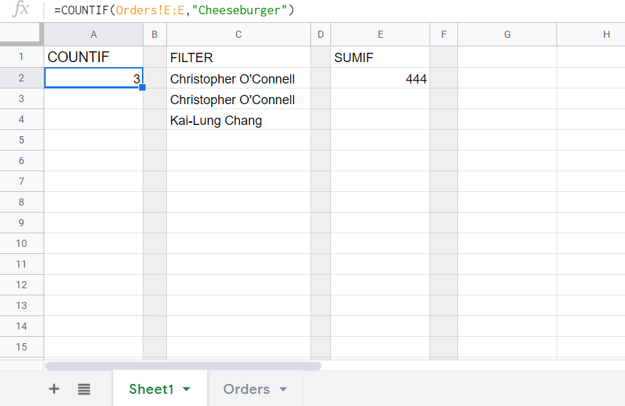
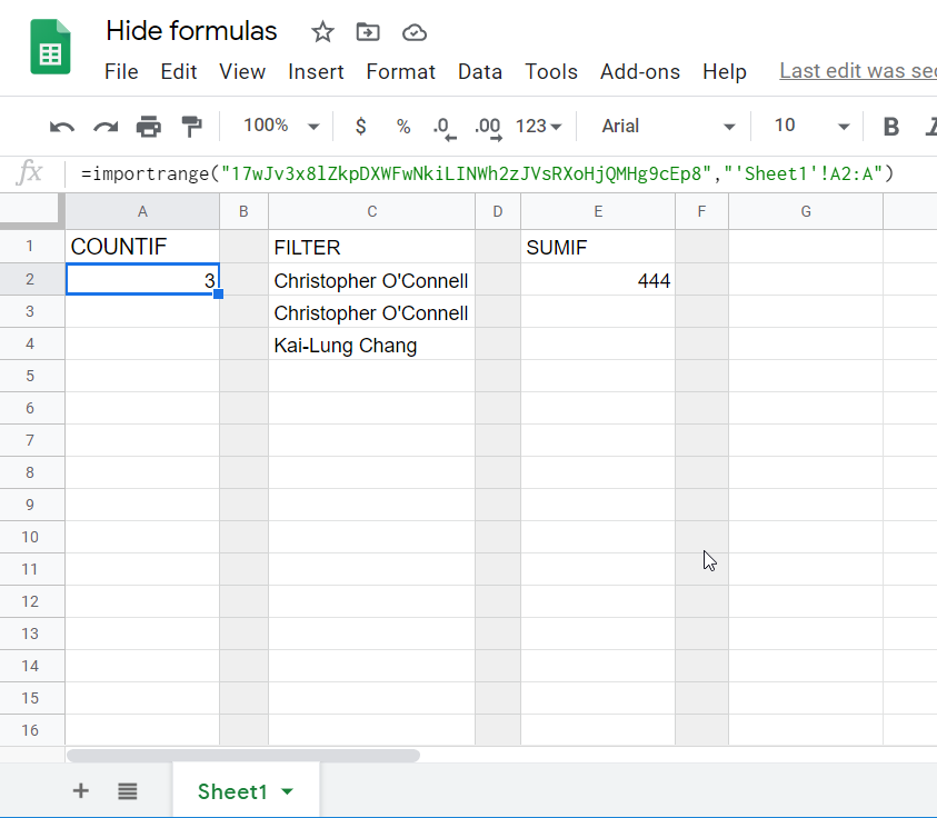
Clone this Google Sheets doc (either make a copy or simply copy and paste data from it) and replace the formulas with the IMPORTRANGE formulas that will reference the original document.

For COUNTIF:

=importrange("17wJv3x8lZkpDXWFwNkiLINWh2zJVsRXoHjQMHg9cEp8","'Sheet1'!A2:A")

For FILTER:

=importrange("17wJv3x8lZkpDXWFwNkiLINWh2zJVsRXoHjQMHg9cEp8","'Sheet1'!C2:C")

For SUMIF:

=importrange("17wJv3x8lZkpDXWFwNkiLINWh2zJVsRXoHjQMHg9cEp8","'Sheet1'!E2:E")

Then connect these sheets, of course. Your spreadsheet will look the same as the original doc. However, instead of the original formulas, you and those you share the spreadsheet with will only see the IMPORTRANGE formulas:

Functions you can use with IMPORTRANGE in Google Sheets

IMPORTRANGE with QUERY in Google Sheets

QUERY+IMPORTRANGE allows you to import data based on certain conditions.

QUERY IMPORTRANGE Syntax:

=QUERY(IMPORTRANGE("spreadsheet", "data_range"), "query_string")

spreadsheet – the URL or ID of the spreadsheet to import data from.
data_range – a range of cells to query.
query_string – a string made using clauses of the Google API Query Language.

This topic has been mentioned above and described in full in our dedicated blog post: QUERY + IMPORTRANGE in Google Sheets.

IMPORTRANGE with VLOOKUP in Google Sheets

VLOOKUP + IMPORTRANGE allows you to import data that matches the specified search criteria. Read more in our blog post VLOOKUP Explained: How to Search Data Vertically in Spreadsheets.

VLOOKUP IMPORTRANGE Syntax:

=VLOOKUP(search_key,IMPORTRANGE("spreadsheet", "data_range"),index,[sorted_boolean])

search_key – the value (or a cell range) to search for.
spreadsheet – the URL or ID of the spreadsheet to import data from.
data_range – a range of cells to query.
index – the index (number) of the imported column in the range to return the value.
[sorted_boolean] – a TRUE/FALSE boolean indicating whether the specified column is sorted. TRUE (sorted) is set by default, but in most cases FALSE is recommended.

For example, we have a spreadsheet with search criteria of specific customer names. The other spreadsheet contains a list of orders per customer. The combination of VLOOKUP and IMPORTRANGE will let us match data across these spreadsheets. Here is the formula:

=vlookup(
   A2:A,
importrange("1iUwZDui3Q6mBpswPuU7e9NdvKwNGRA9A3JAhqFDMFbk","All orders!C2:I"),
   3, false)

If you modify the formula above by adding the ARRAYFORMULA function and IF + LEN, you’ll get the following:

=arrayformula(
  if(len(A2:A)=0,,
   vlookup(
    A2:A,
  importrange("1iUwZDui3Q6mBpswPuU7e9NdvKwNGRA9A3JAhqFDMFbk","All orders!C2:I"),
    3, false
   )
)

Read our Guide of Using ARRAYFORMULA in Google Sheets For All.

IMPORTRANGE with FILTER in Google Sheets

FILTER + IMPORTRANGE allows you to filter the imported data by a certain value.

FILTER IMPORTRANGE Syntax:

=FILTER(IMPORTRANGE("spreadsheet", "data_range"),[condition_1, condition_2,...])

spreadsheet – the URL or ID of the spreadsheet to import data from.
data_range – a range of cells to query.
condition – a range that contains the filter criteria.

For example, we need to import a data range from a spreadsheet and filter it by a specific product name: “Denver sandwich“. Here is how it may look:

=filter(
importrange("1iUwZDui3Q6mBpswPuU7e9NdvKwNGRA9A3JAhqFDMFbk","All orders!C2:I"),
importrange("1iUwZDui3Q6mBpswPuU7e9NdvKwNGRA9A3JAhqFDMFbk","All orders!E2:E")="Denver sandwich"
)

importrange("1iUwZDui3Q6mBpswPuU7e9NdvKwNGRA9A3JAhqFDMFbk","All orders!C2:I") – data range to import
importrange("1iUwZDui3Q6mBpswPuU7e9NdvKwNGRA9A3JAhqFDMFbk","All orders!E2:E") – a column from the imported data range where the filter criteria is
"Denver sandwich" – filter criteria

Read the FILTER Function Tutorial to learn more about filtering in Google Sheets.

IMPORTRANGE with SUM in Google Sheets

SUM + IMPORTRANGE allows you to sum the imported data range.

SUM IMPORTRANGE Syntax:

=SUM(IMPORTRANGE("spreadsheet", "data_range"))

spreadsheet – the URL or ID of the spreadsheet to import data from.
data_range – a range of cells to query.

For example, we need to import a column from a spreadsheet and return the sum of its values. Here is the formula:

=sum(importrange("1iUwZDui3Q6mBpswPuU7e9NdvKwNGRA9A3JAhqFDMFbk","All orders!I2:I"))

IMPORTRANGE with SUMIF in Google Sheets

You can’t use the IMPORTRANGE function within a SUMIF formula. If you need to sum a range from a spreadsheet according to a set criteria, you can do one of the following:

Use QUERY+IMPORTRANGE
Import the data with IMPORTRANGE, then apply SUMIF to the already imported data.

These are the most popular inquiries of Google Sheets functions to combine with IMPORTRANGE. If you know other in-demand cases, mention them in the comments section below, so we may include them in the blog post.

IMPORTRANGE or Google Sheets integration by Coupler.io?

You should select the option to import data from Google Sheets documents based on your requirements:

IMPORTRANGE works well if you need to import smaller amounts of data. However, this Google Sheets function is limited in functionality, requires a lot of manual work, and can slow the productivity of your spreadsheet if many IMPORTRANGE formulas are applied.
Coupler.io is a stable solution that can handle large amounts of data and multiple calculations in a single document. Moreover, this Google Sheets add-on lets you automate data import across spreadsheets on schedule.

Check out the following comparison table to make the final decision:

Google Sheets integration		IMPORTRANGE
Web app and a Google Sheets add-on	Entity	Google Sheets function
Google Spreadsheets limits or Google Sheets API limits	Limitation	Max 50 connections per spreadsheet
– Specified data range on a single sheet – Entire sheet – Consolidation of sheets of a spreadsheet	Data to import	– Specified data range on a single sheet – Consolidation of sheets of a spreadsheet
Automatic and manual options are available	Data refresh	Automatic within a few seconds
Available	Scheduled refresh	Not supported
No limitations	Data availability	When you open the spreadsheet
Available	Append imported data	Not supported

Choose the best solution for your project and good luck with your data!

Import data to Google Sheets with Coupler.io

Get started for free

Exit mobile version