How to Transform Data in Excel? Ultimate Guide

Excel is a popular and handy tool for storing mathematical, statistical, and other information. Does Excel provide any functionalities for data transformation? Of course, it does! To transform data in Excel, you can use multiple functions, as well as native and third-party tools to automate processes. Read on to learn about all the available options. 

What is data transformation in Excel?

According to Wikipedia:

Data transformation is the process of converting data from one format or structure into another format or structure.

So, you basically change the format without changing the information content of the data. The goal of data transformation is to present the data so that it can be used most effectively.

Data transformation in Excel means the same process but implemented in Excel and with the help of Excel functions and tools. For example, you can remove a column, change the data type, or filter rows. Each of these operations means data transformation. 

What can you use to transform data in Excel?

Suppose you are planning to transform data values ??in Excel. In that case, you can take advantage of the numerous Excel functions, as well as built-in and third-party tools.

Excel functions

As for data transformation, Excel itself has a vast number of functions that allow you to transform data, change the spreadsheet’s appearance, perform various mathematical operations, and many others. These functions are more than enough to help you structure and organize your data in most simple cases.

Power Query

Power Query is a popular Excel tool used to extract, transform, and load data. It can be used as part of a self-service ETL solution to perform the following tasks:

• Extract data from the source.
• Transform your data to prepare it for analysis.
• Load the transformed data into a worksheet or data model.

Power Query lets you define transformation steps such as removing duplicates, splitting columns, or changing data types. Once set up, these steps run with each refresh, and keep your data consistent for recurring reports.

That said, the refresh isn’t automatic. You’ll need to trigger it manually unless you’ve configured advanced automation. Power Query also has a learning curve, as it introduces concepts like queries, applied steps, and its own formula language that differs from standard Excel functions.

Power Pivot

This is an Excel-like user interface to a full-fledged SQL database installed on your computer and is a powerful tool for processing vast amounts of data. Power Pivot allows you to:

• Link imported spreadsheets by key columns.
• Filter and sort them.
• Perform mathematical and logical operations using more than 150 functions of the built-in DAX language.

Power View

Power View made its way into Excel 2013 from SharePoint. It primarily provides the user with tools for quickly creating live visual reports using pivot spreadsheets and database-based charts.

You can add totals to the report in a simple spreadsheet, a pivot spreadsheet, and various types of charts. Power View allows you to link data from spreadsheets even to Bing maps.

Coupler.io

Coupler.io is a reporting automation solution that helps you keep your Excel reports updated with fresh and ready-to-use data without manual effort. It connects with 60+ data sources and allows you to schedule automatic data transfers into Excel at hourly, daily, or custom intervals.

But Coupler.io goes beyond just moving data. It also lets you transform your data during the transfer process, so the spreadsheet has clean, organized, and structured data for analysis. Below are the data transformation features in Coupler.io:

• Hide, rename, and reorder columns to match your reporting structure.
  
• Change column types and formats such as text, number, date, or boolean.
  
• Filter rows based on conditions using AND/OR logic for more precise results.
  
• Sort data by any column in ascending or descending order before import.
  
• Add formula-based columns to calculate new metrics using existing data.
  
• Summarize data with aggregation functions like sum, average, or count.
  
• Append data from multiple sources by stacking rows with matching columns.
  
• Join datasets using a shared column to combine related data from different sources.

These features make it easier to work with organized and analysis-ready data without spending extra time formatting it manually in Excel.

You can explore the full list of Excel integrations Coupler.io supports and set up imports that fit your needs.

What are the data transformation functions in Excel?

There are a considerable number of Excel data transformation functions. Here are 10 of the most popular ones:

Function	Description
LOG10	Allows you to calculate the logarithm to base 10.
ASIN	Allows you to calculate the arcsine.
SQRT	Allows you to calculate the square root.
ABS	Returns the absolute value of a number
LET	Assigns names to the results of calculations to allow storage of intermediate calculations, values, or name definitions in a formula.
ARABIC	Converts Roman numerals to Arabic numerals as a number.
DATE	Returns the sequential serial number that represents a particular date.
DAYS	Returns the number of days between two dates.
DEGREES	Converts radians to degrees.
ISO.CEILING	Rounds a number up to the nearest integer or multiple.

Each function can perform one or more actions. You are unlikely to have to use all the existing functions. On average, one person uses 3 to 10 different functions, depending on what field of activity they work in.

Example of transforming data in Excel

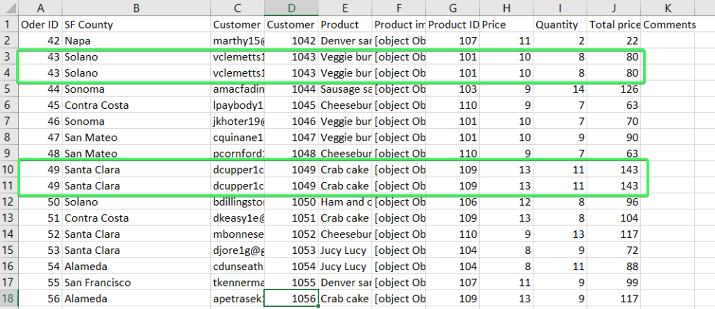
One of the simplest examples of data transformation in Excel is removing duplicates. In Excel, you can do this either with Power Query if you’re getting data from an external source or with a button if your data set is already in Excel. Here is an example of a data set with duplicate records.

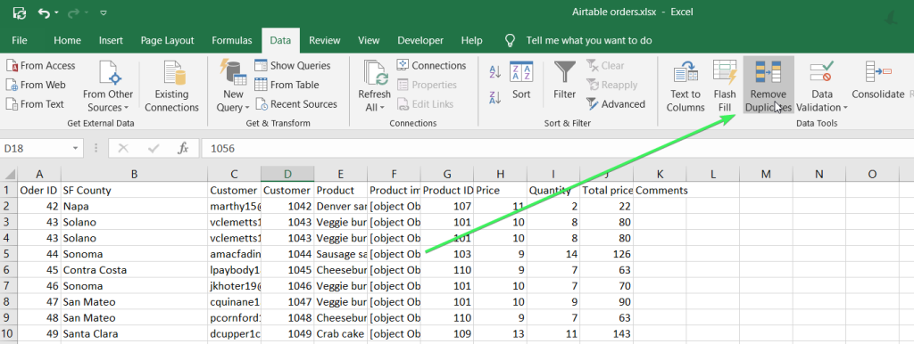
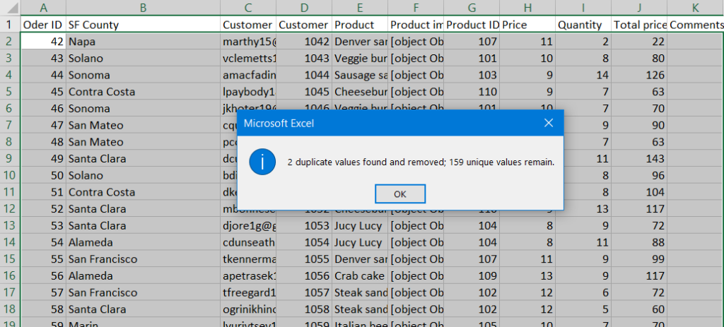
To remove these duplicates, click the Remove Duplicates button on the Data tab, then select the columns that contain duplicates.

There you go!

Removing duplicates from multiple sources with Coupler.io

However, it becomes complicated when your data comes from multiple sources. For example, let’s say you’re importing leads from HubSpot and the information about webinar registrations from Google Sheets. It can be easily done with Coupler.io, which lets you import and blend data from these sources. You might have overlapping records but with slight differences like 

• Inconsistent capitalization: ‘John Doe’ is capitalized in HubSpot but is in lower case ‘john doe’ in Google Sheets data.

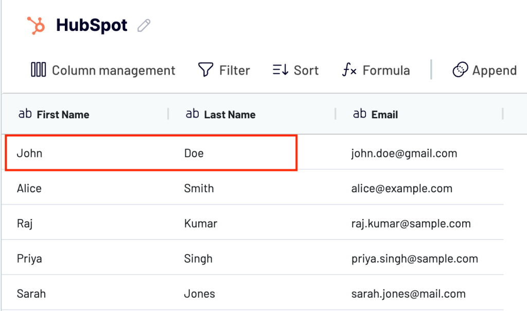
• Extra spaces in email addresses: There is an extra space after ‘john.doe’ in the email address field. 

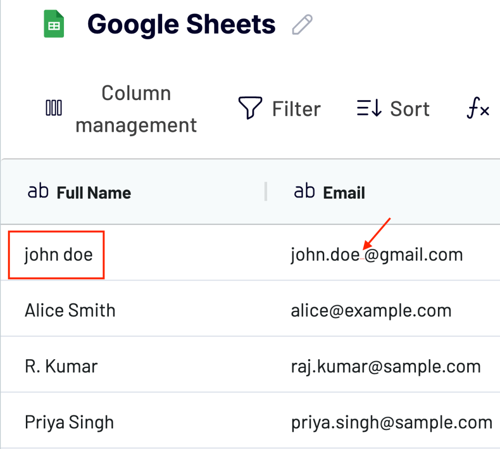
Because of this, when we try to join the data from these two sources, the First Name, Last Name, and Email of the lead are missing.

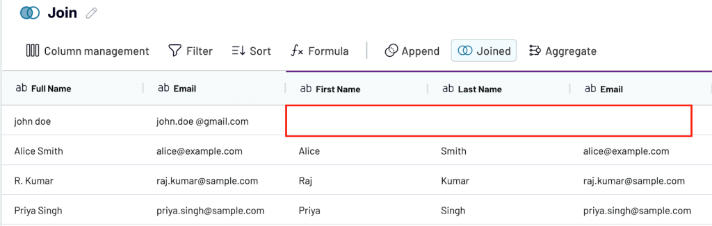
In such cases, Excel cannot recognize them as duplicates.

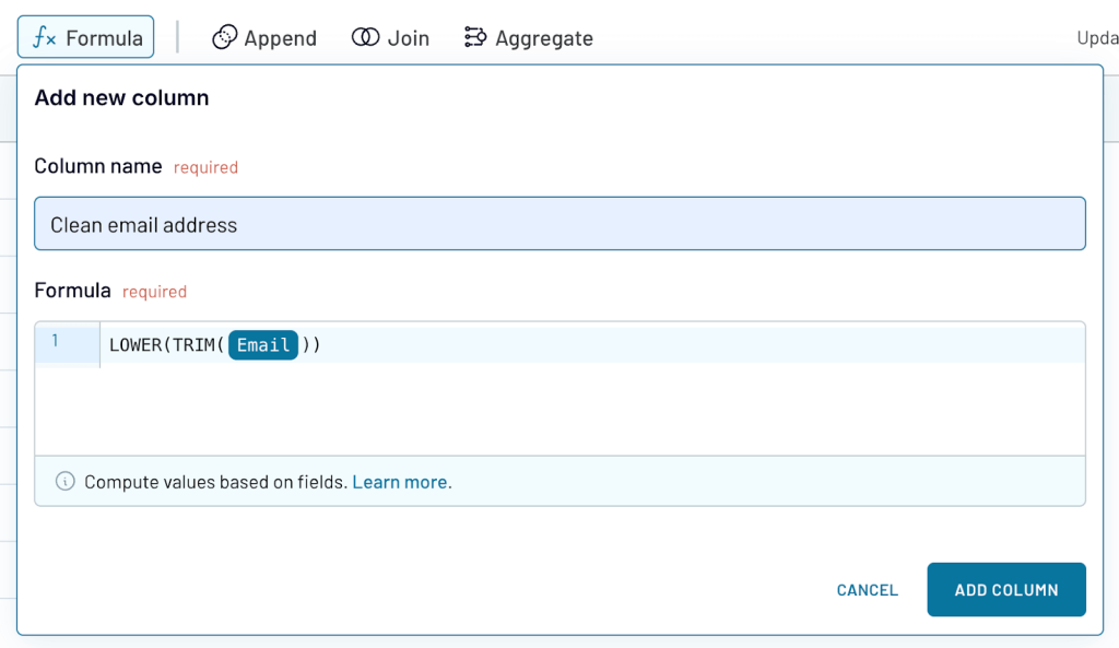
But with Coupler.io’s data transformation features, it is easy to handle this during the import process. You can:

• Use formulas like LOWER(TRIM(email)) to clean email addresses

• Create a new Full name column combining first name and last name
• Filter out incomplete or irrelevant rows (if any)

Now you can see a clean and well-formatted dataset that looks like this. The names are all lowercase and neatly trimmed. 

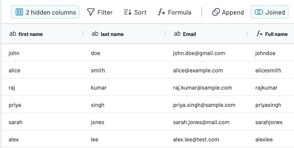
These small steps during the import process make deduplication. It’s a great way to maintain clean and accurate reports without spending time fixing them manually. Does it look fancy to you? Learn what other data transformation options Coupler.io can offer.

Import and transform data in Excel with Coupler.io

Start by selecting the source app from the drop-down in the form below and click Proceed to load data from your cloud source to Microsoft Excel. You can sign up for free with no credit card required.

Configure the source connection following the in-app instructions. You can also add multiple sources to blend data into a single output after that.

Once your source accounts are connected and configured, move to the next step: Transformations. Here, you can organize and prepare your data before it is transferred to Excel:

Column management

Hide columns you don’t need, rename them for better readability, and reorder them to match your preferred structure. 

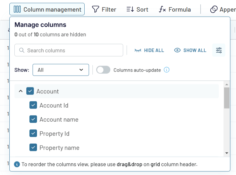
You can also change the column type (like number, date, or boolean) and define formats such as decimal precision or time zone.

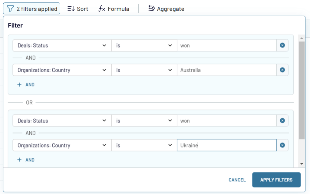
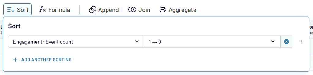
Sort and filter

Depending on the data type, apply filters like contains, is empty, greater than, or starts with. You can also combine multiple filters using AND or OR logic to narrow down the dataset.

To organize your reports before the data even lands in Excel, sort your data by any column in ascending or descending order.

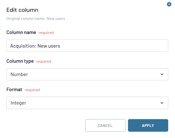
Custom formulas

Create custom columns by using formulas on existing fields. For example, calculate the views-to-new-users ratio or add percentage-based metrics directly within the import setup.

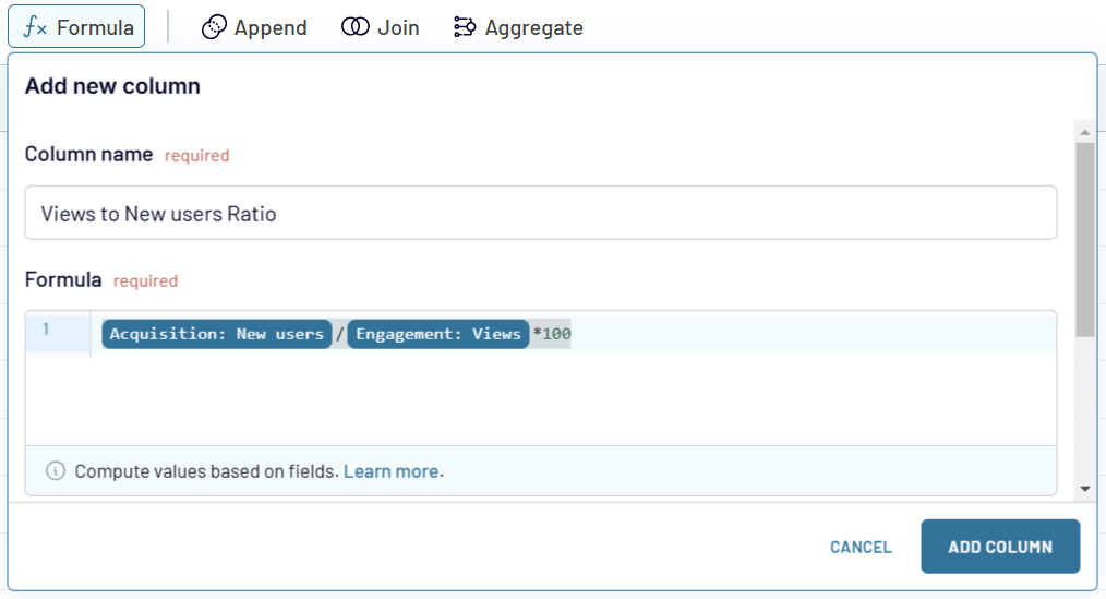
Functions like LOWER, TRIM, and arithmetic operations can be combined to clean or enhance your data. Added columns can be edited or deleted, giving you full flexibility during import.

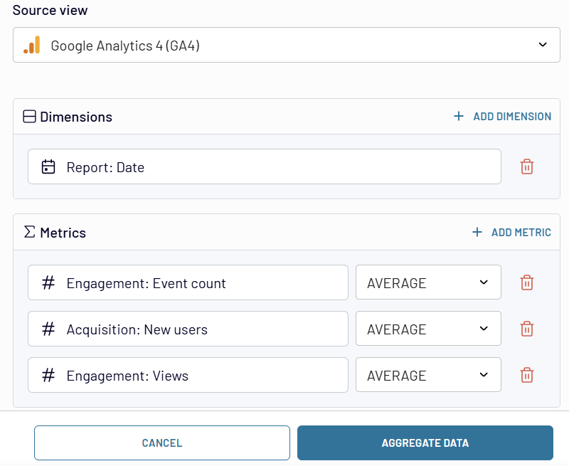
Aggregation 

Perform summary calculations like sum, average, count, min, or max. Group your data by one or more fields (like region or product name) to create a high-level overview.

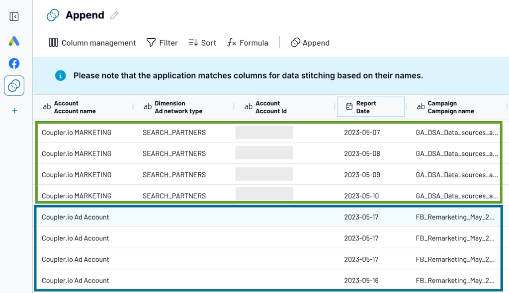
Append and Join 

Stack data using Append from multiple sources with similar structures into a single table. Columns with matching names are merged automatically, while unmatched ones are added alongside. For best results, align column names like “Impressions” or “Conversions” across sources before appending.

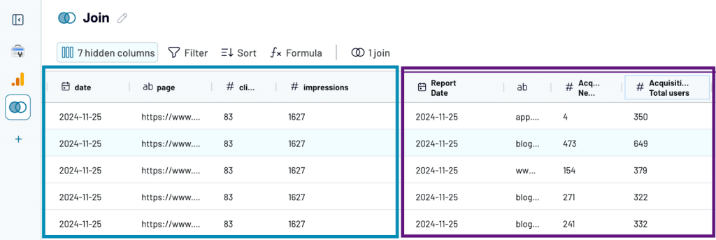
Use the Join feature to combine two datasets with different structures using a common field, which is usually a dimension, such as “Date” or “Campaign.” All rows from the main dataset are kept, and only matching rows from the secondary source are added. You can join multiple sources and reuse the result in other transformations or reports.

Once your data is transformed, follow the in-app instructions to configure Excel as the destination. 

Next, set up an automatic refresh schedule that fits your needs. You can choose to update your Excel file hourly, daily, or at a custom interval. This makes sure your reports stay up to date without manual intervention.

Import and transfrom your data with Coupler.io

Get started for free

Examples of transforming data using Excel functions and tools

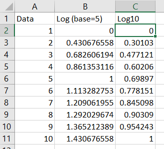
How to transform data into log in Excel?

Users working with stats or scientists or other researchers need to calculate the logarithm of a certain number. It can be quickly done if you use a calculator, but what if there is a large amount of data, and you need to do everything as soon as possible? Then, use log transform data in Excel. To convert the required data to a logarithm, you can use two functions: LOG and LOG 10.

• LOG10 is the function to return the base-10 logarithm of a number.

=log10(number)

• LOG is the function to return the logarithm of a number to the base you specify. The default base value is 10.

=log(number,base)

For example, here are two log transform formulas:

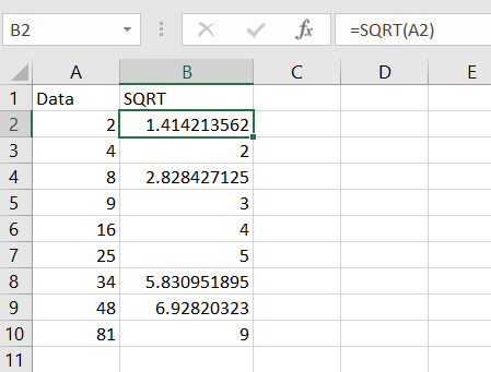
How to square root transform data in Excel?

To apply the square root transformation to a data set in Excel, you can use the SQRT function.

=SQRT(number)

For example:

How to make cube root Excel data transformation?

There is no dedicated function in Excel for cube root transformation. However, you can apply the following formula:

=[value]^(1/3)

For example:

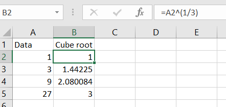
According to this principle, you can perform root transformations of any degree, replacing 3 with the degree you need.

How to arcsine transform data in Excel?

The arcsine is the angle whose sine is the number. The arcsine transform can be used to stretch points between 0 and 1, for example, when working with proportions or fractions. 

The arcsine transformation or the angular transformation is calculated as two times the arcsine of the square root of the proportion. To transform such data, use a combination of two functions: ASIN, which returns the inverse sine of a number, and SQRT.

=ASIN(SQRT())

For example, it looks like this:

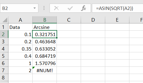
The formula only works for the values in the range from 0 to 1. For example, it returned a #NUM! error for value 2. To avoid this, you will need to convert values to fit the 0 to 1 range. For this, divide each value by the max value into the data set using the following formula:

=[value]/MAX([data-set])

For example:

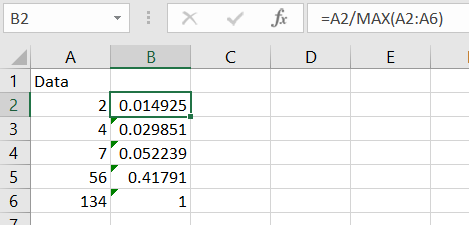
Nest this formula with the arcise one and you’ll get the proper result, for example:

=ASIN(SQRT(A2/MAX(A2:A6)))

How to transform data in Excel from columns to rows?

Use the transpose function if you have a worksheet with data in columns that need to be rotated to change its row order. With it, you can quickly switch data from columns to rows or vice versa.

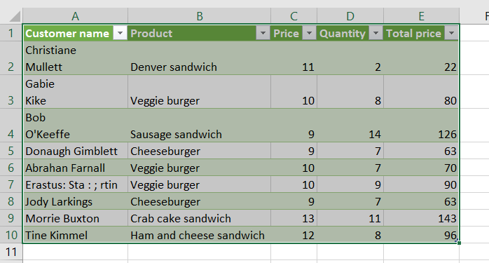
Suppose you had a data set like this:

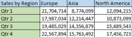
The transpose function rearranges the data set so that it looks like this:

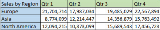
To perform this transformation, you should select the range of data you want to reorder, including any row or column labels, and press Ctrl+C.

Next, you need to select a new location on the worksheet to insert the transposed data set (make sure you have enough space). The new data set that you insert here will completely overwrite any data/formatting already there.

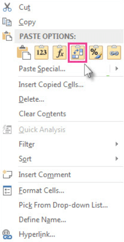
Right-click the top-left cell to paste the transposed data set, then select Transpose.

Once you’ve transformed data in Excel, you can delete the original data set, and the data in the new one will remain intact.

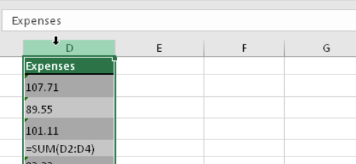
How to transform into numeric data in Excel?

Sometimes, data in Excel is textual, which can lead to some problems. Fixing this is easy enough. You should select the cells and click on the diamond icon with an exclamation mark to select the conversion option to get started. You can perform such actions if this button is not available.

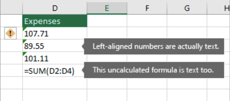
You should select the column where this problem occurs (if you don’t want to convert the entire column, you can select multiple cells instead).

On the Data tab, click Text to Columns.

The Text to Columns button is typically used to split a column, but it can also be used to convert a single column of text to numbers.

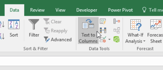
The remaining steps of the Text to Columns functionality are best for splitting a column. Since you’re just converting text in a column, you can click Apply right away, and Excel will convert the cells.

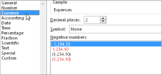
Press CTRL + 1 (or ? + 1 on Mac). Then choose any format.

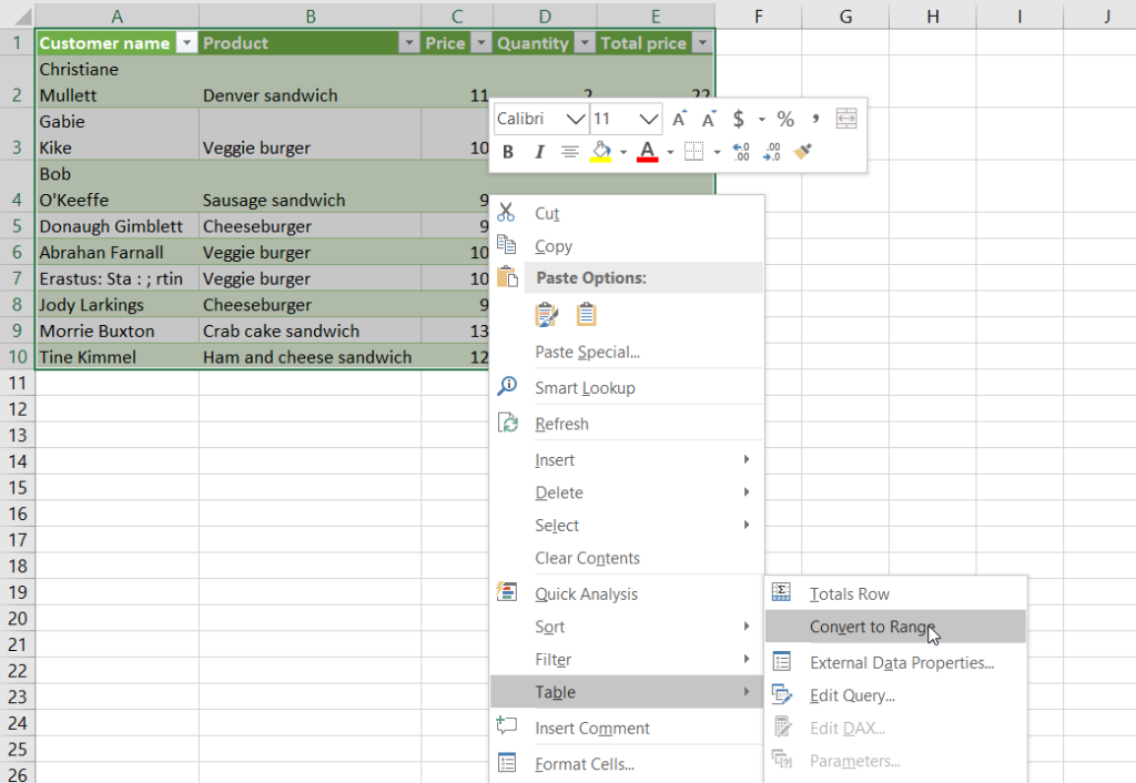
How to transform data range in Excel?

At any moment, you can convert the table to a normal range of data on a worksheet.

Right click on the table, select Table => Convert to range.

But when you’re working with multiple datasets from different tools, things can get a bit messy.

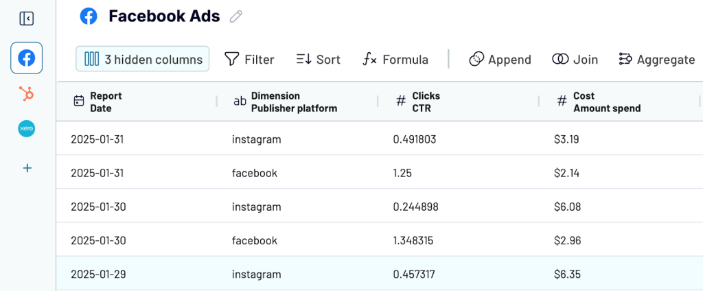
Let’s say you’re using data from Facebook Ads, HubSpot, and Xero. You might want to track how ad leads move through the sales pipeline and how they translate into actual revenue. Managing this manually in Excel is time-consuming.

With Coupler.io, you can automate it. You can pull each dataset into separate sheets within the same Excel workbook or blend and transform the data before sending it over, depending on what kind of analysis you need.

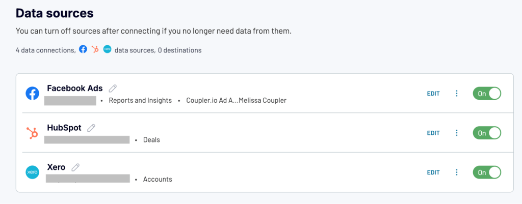
This makes it easy to build a full-funnel view. You’ll be able to see which campaigns brought in leads, how those leads progressed through deals, and how much revenue was actually collected.

In what cases may data transformation in Excel be needed?

Often, simply arranging data alphabetically, in ascending order, or transforming non-normal data in Excel is not enough. To understand the information, sometimes more complex transformations are required.

After conducting any sociological research, the collected data needs to be grouped in one place, and a detailed analysis should be carried out. Entrepreneurs use Excel data transformation to create reports or optimize their work. These can be companies that are engaged in sales or even tour operators. 

If we talk about mathematics or physics, the systematization of data allows them to simplify the work as much as possible. And if, when working with data, you can immediately calculate the square root or raise a number to a power, it makes the work faster. It is almost impossible to list all areas where data transformation in Excel can be used, but to name a few:

• Reporting
• Analysis of statistical data
• Performing mathematical operations with a large amount of data
• Compiling financial data
• Business analytics, and many others

Each specialty can use data transformation in different ways, depending on their goals and needs. 

Main ideas for data transformation in Excel

The value of data transformation in Excel is difficult to overestimate.  It can be used in various fields, such as sociology, mathematics, physics, and many other sciences. It solves several problems:

• Transforms data so that it is easier to do calculations
• Allows you to modify tables so that it is more convenient to work with them
• Simplifies data analysis
• Facilitates the creation of various reports and monitoring

Sometimes, it is impossible to perform calculations correctly since the values can be measured in different physical quantities (for example, radians and degrees), or vice versa; we need to perform some rounding. To not do all the conversions manually, you can use the special features of Excel. It allows you to save a lot of time, effort, and energy to deal with more complex and important processes, while computer technology is doing monotonous work.

Basic Excel data transformation rules

When transforming data in Excel, you need to remember the rules for using this spreadsheet:

• Any action can be reversed, so you should never panic.
• Using formulas when working with Excel simplifies working with a spreadsheet, but if you wish, you can do without them in some cases.
• If you work with Google Excel, there is no need to save permanently, but the interface and functions may differ slightly.
• Some add-ons may already be built into your version of the spreadsheet, while others may need to be downloaded. In the second case, use only trusted sites to avoid downloading a computer virus.

The above rules are not complex, and you can easily remember them even before working with a spreadsheet.

Data transformation workflows

Transforming data is not just applying a filter or adding a custom formula.  A data transformation workflow involves several steps: 

• Importing raw data
• Formatting it
• Adding transformations
• Analyzing or visualizing the results

While Excel can handle each of these tasks individually, manually managing them on a recurring basis is time-consuming and error-prone.

Coupler.io makes it easier by building an automated and repeatable workflow that allows you to:

• Import data from 60+ sources: You can pull data from CRM apps like HubSpot, ad platforms like Facebook Ads, accounting tools like Xero, project management systems like Jira or Trello, and many others. All your tools can feed into one central Excel workbook without manual exporting or copy-pasting data.
  
• Apply transformations using SQL queries or pre-built templates: Clean and prepare your data as it’s being imported. From filtering rows and formatting fields to blending data and applying custom formulas, you can transform your data the way you need it.
  
• Refresh data on a schedule that works for you: Set automatic updates to run hourly, daily, or on a custom schedule. This keeps your reports and dashboards up to date, with no manual effort.
  
• Keep a version history of your data: Every import is tracked, so you can easily view or restore previous versions if something changes or breaks. It’s a simple way to keep your data process transparent and reliable.
  

For example, let’s say you manage inventory and finances across tools. Your product catalog is stored in Airtable, orders are tracked in Google Sheets, and expenses are logged in QuickBooks. 

Instead of switching between platforms and collecting data manually, Coupler.io pulls all of it into a single Excel workbook—structured, cleaned, and refreshed on a schedule you set.

Automate data load to Excel with Coupler.io

Get started for free

What to do if transform data in Excel fails?

Even with the right tools, things can occasionally go wrong during the transformation process. A formula might break, a large file might crash, or important data might get lost along the way.

To avoid these issues, it’s good to have a backup strategy in place. You can store copies of your data in another Excel workbook, sync it to the cloud, or even export it to tools like Google Sheets or a data warehouse like BigQuery.

Coupler.io makes this process efficient by allowing you to automate your backups. You can set your data to export on a regular schedule (hourly, daily, or weekly), so you always have the latest version saved and ready to restore if needed.

And, it is more than just backups. Since Coupler.io handles data transformation in the cloud, you can offload the heavy lifting like filtering, cleaning, or combining large data sets, before anything is imported into Excel. You’ll be working with already-structured data, which helps keep your spreadsheets lightweight, responsive, and less prone to crashing.

Building a reliable transformation workflow outside of Excel can make a big difference in saving time, reducing risk, and keeping your Excel reports running smoothly.

Zakhar Yung

A content manager at Coupler.io whose key responsibility is to ensure that the readers love our content on the blog. With 5 years of experience as a wordsmith in SaaS, I know how to make texts resonate with readers' queries??