VLOOKUP Function in Excel: Overview, Step by Step Guide, Examples and Troubleshooting

When you learn the price of the menu below, first your eyes will look up vertically to find your favorite pie, such as The Mushroom Lover. Then your vision slides to the right to find the price for the L size – $27.99.

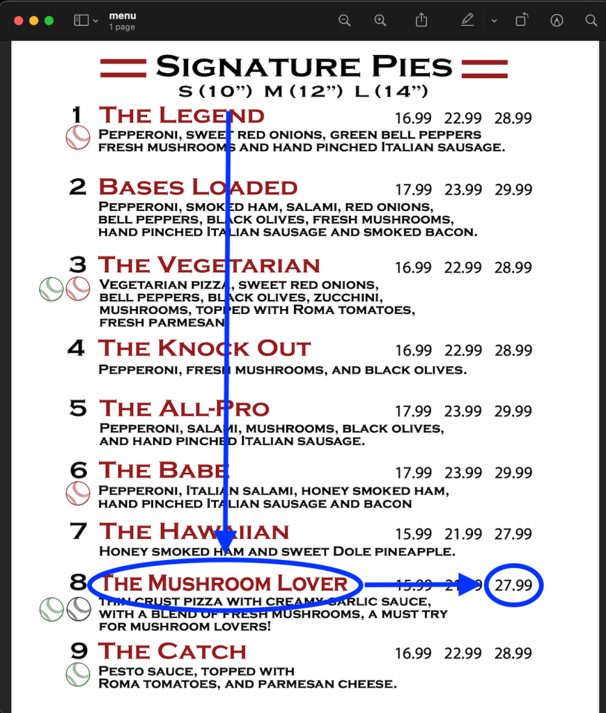
You’ve just done a vertical lookup, or vlookup. For this purpose, spreadsheet apps including Excel usually provide a specified function called VLOOKUP. In this article, we’ll explore how you can use the Excel VLOOKUP function, check out a few examples, and learn how to troubleshoot it. 

What is VLOOKUP in Excel

VLOOKUP stands for vertical lookup. It is a function in Excel that searches vertically a specified value in a column to return a matching value, or values in the same row from different columns. 

VLOOKUP syntax in Excel

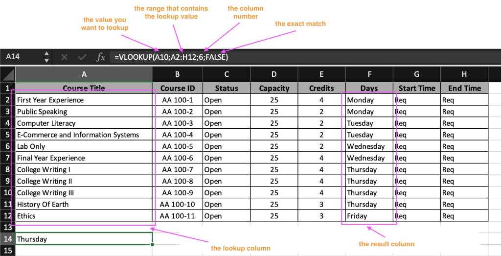
=VLOOKUP("lookup_value",lookup_range, column_number, [match])

• "lookup_value" is the value you want to look up vertically. Quotes are not used if you reference a cell as a lookup value.
• lookup_range is the data range where you’ll search for the lookup_value and the matching value. 
• column_number is the number of the column in the lookup_range, which contains the matching value to return. For example, if your range is D7:G18, D is the first column, E is the second one, and so on.
• [match] is the optional parameter to choose either closest or exact match. To return the closest match, specify TRUE; to return an exact match, specify FALSE. The closest match (TRUE) is set by default.

How to VLOOKUP in Excel – formula example

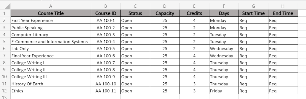
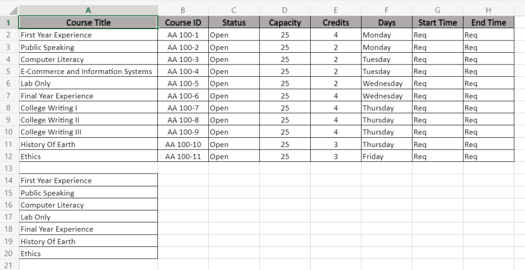
We have the following dataset with the details of courses:

Let’s search for the day when College Writing III is scheduled. Here is the VLOOKUP formula to do this:

=VLOOKUP(A10,A2:H12,6,FALSE)

• A10 – the lookup_value “College Writing III“
• A2:H12 – the lookup_range
• 6 – the column number to return the matching value from
• FALSE – the exact match to return

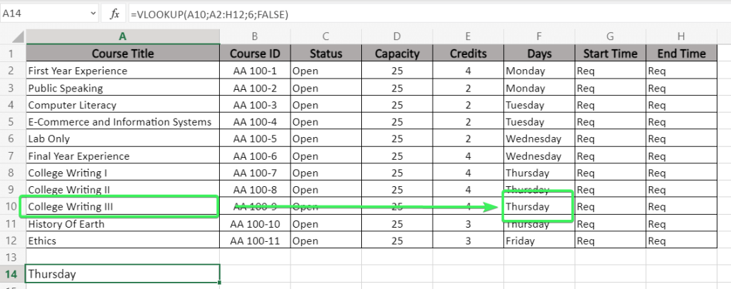
The result of the schedule for College Writing III is Thursday. And here is how the logic of this VLOOKUP formula looks:

• Excel searches the value of A10 (College Writing III) in the lookup column (A2:A12).
• If the value is found, Excel moves across the row to column number 6 of the specified data lookup range (A2:H12). Column A is the first column in the lookup range, because column A contains the lookup value.
• As the formula is set to FALSE (to find the exact match) then the return value is Thursday (you can see the result in A14).

What you should know about VLOOKUP in Excel

• The VLOOKUP function executes a case-insensitive lookup.
• Excel VLOOKUP returns a #N/A if the lookup_value is not able to be found inside the lookup_range.
• Excel VLOOKUP returns a #VALUE! error if the value of column_number is less than 1.
• Excel VLOOKUP returns a #REF! error if the value of column number is greater than the number of columns in the lookup_range.
• The closest match (TRUE) is specified by default.

How to pull your data to Excel for vertical lookup 

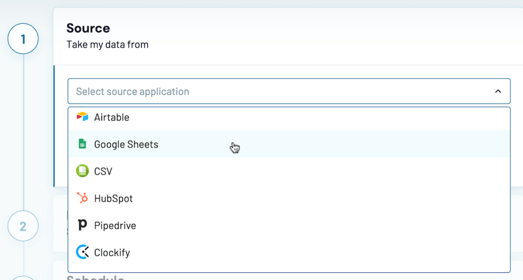
The example above is basic for you to understand the logic of the Excel VLOOKUP function. Your cases probably will be more advanced for the data that you can import from different sources to Excel. How? Coupler.io, an integration solution, is designed to export data from multiple apps and sources to Excel or Google Sheets or BigQuery on a schedule. You just need to sign up to Coupler.io and:

• Select and set up a source:

Check out the HubSpot to Excel integration.

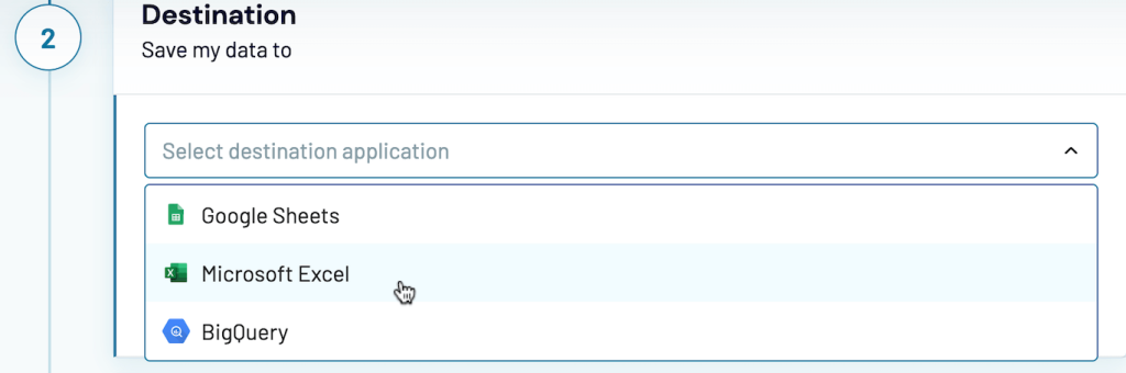
• Select and set up a destination (in our case – Microsoft Excel)

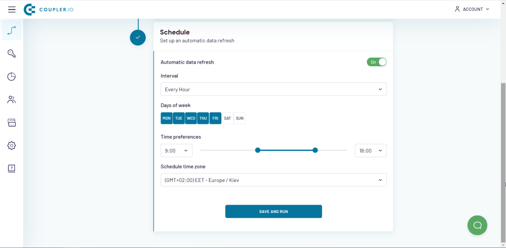
• Set up a schedule (optionally) if you want to automate export of your data on a custom schedule.

With your data exported from BigQuery, HubSpot, Xero, etc. to Microsoft Excel, you can easily vlookup it.

How to use VLOOKUP in Excel

There are two ways to access VLOOKUP in Excel – you can use the VLOOKUP formula in the formula bar or access it through the menu bar.

Type directly into the cell

In the example above, we used VLOOKUP in Excel this way. You need to click in the cell where you want the answer to appear, then put the cursor on Formula Bar. Type the VLOOKUP formula and all its parameters directly into the formula bar:

Using menu bar

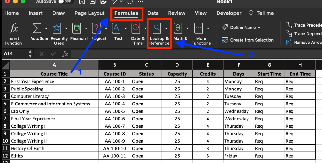
• In the menu bar, select the Formulas tab, then select Lookup & Reference.  

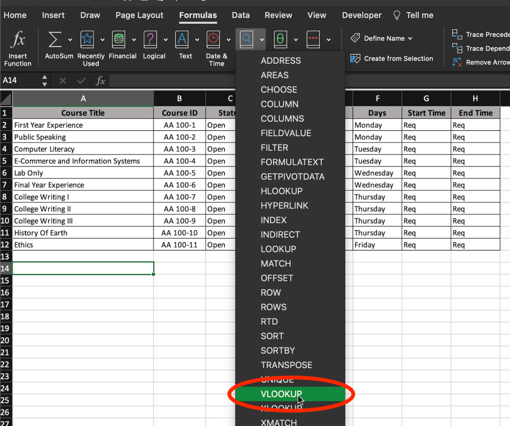
• An alphabetical menu will drop down – choose VLOOKUP. 

• On your right side, the Formula Builder will appear.

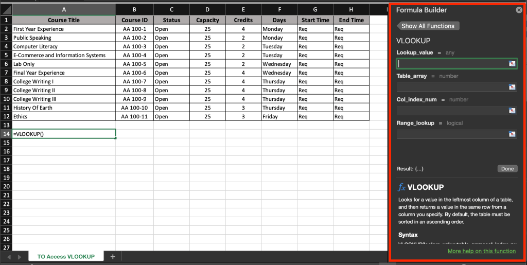
• Fill each box in the Formula Builder as your VLOOKUP formula parameters, then click Done.

Here is how it will look for our Vlookup formula example:

The result is the same – Thursday. So it is up to you which way is easier for you to use the VLOOKUP function 🙂

Excel VLOOKUP for an array

In the Excel VLOOKUP, you can use an array as a lookup_value. This will let you search the matches for multiple values. 

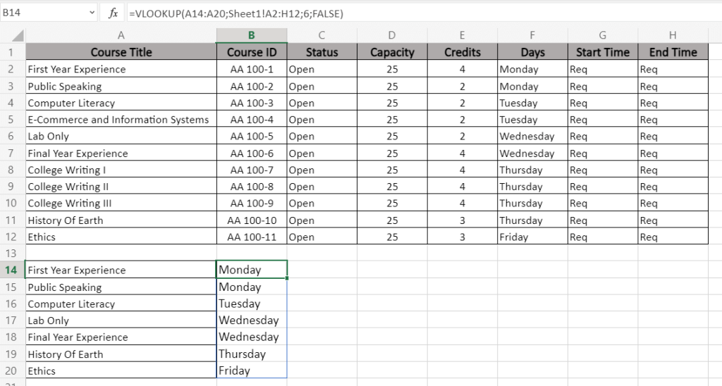
Let’s take the data set from above and vertically look up for the days when the values from the range A14:A20 are scheduled. 

Here is the VLOOKUP formula to do this:

=VLOOKUP(A14:A20,Sheet1!A2:H12,6,FALSE) 

• A14:A20 – the lookup array
• Sheet1!A2:H12 – the lookup range
• 6 – the column number to return the matching value from
• FALSE – the exact match to return

Excel vlookup cases

Check out the following specific cases of how to vlookup data in Excel:

• How to VLOOKUP for multiple matches
• How to VLOOKUP for two values
• How to VLOOKUP for multiple criteria
• How to compare two columns in Excel using VLOOKUP
• How to VLOOKUP another sheet in Excel 
• How to vlookup another workbook/spreadsheet in Excel
• How to vlookup multiple columns in Excel
• Excel SUMIF with VLOOKUP

Excel reverse VLOOKUP

VLOOKUP in Excel can only look up the matching values from left to right. 

And what if your data set look like this and you need to look up values from right to left:

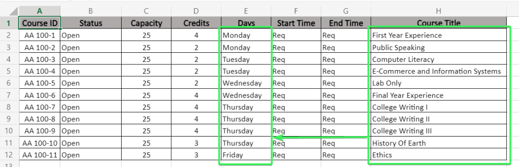
Unfortunately, in this case you can’t use VLOOKUP, but the Excel XLOOKUP function will do the job. 

Note: The XLOOKUP function is only available in Excel Online and Microsoft 365.

Reverse VLOOKUP syntax

=XLOOKUP("lookup_value", lookup_array, return_array, "[if_not_found]", [match_mode], [search_mode])

• lookup_value is the value you want to look up vertically.
• lookup_array is the data array to search the lookup_value. 
• return_array is the data array to return the matching value.
• [if_not_found] is the optional parameter to return a specified text if the lookup_value has not been found.
• [match_mode] is the optional parameter to choose the match mode:
  • 0 – Exact match (default)
  • -1 – If the exact match is not found, the next smallest item is returned.
  • 1 – If the exact match is not found, the next largest item is returned.
  • 2 – A wildcard match where *, ?, and ~ have special meaning.
• [search_mode] is the optional parameter to choose the search mode:
  • 1 – Search starting at the first item (default).
  • -1 – Search starting at the last item.
  • 2 – Binary search that relies on lookup_array being sorted in ascending order. If not sorted, invalid results will be returned.
  • -2 – Binary search that relies on lookup_array being sorted in descending order. If not sorted, invalid results will be returned.

Reverse VLOOKUP formula example

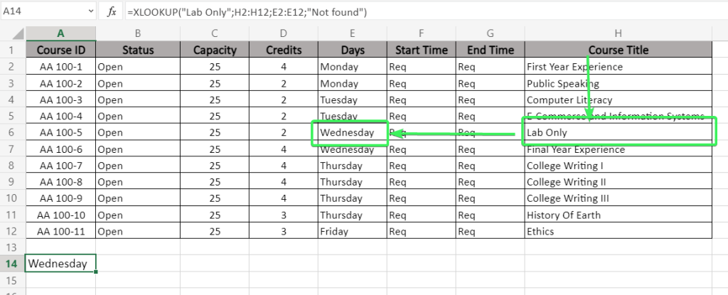
Let’s search for the day when Lab Only is scheduled. Here is the XLOOKUP formula to do this:

=XLOOKUP("Lab Only",H2:H12,E2:E12,"Not found")

• "Lab Only" – the lookup value.
• H2:H12 – the data array to search for the lookup value
• E2:E12 – the data array to return the matching value.
• "Not found" – the text to return if the lookup value has not been found.

Another way to do a reverse vlookup is using a combination of the INDEX and MATCH functions, please see this section to learn about these functions.

If your VLOOKUP formula is not working in your Excel

Sometimes when you use VLOOKUP, the #N/A error message appears. It is the most dreaded and trickiest to handle. Here, we give the five most common reasons why your VLOOKUP is not working, including the solution for each case.

#1: Exact match in the VLOOKUP formula is not specified

Issue

On the following screenshot, we have a VLOOKUP formula, which returns an incorrect result. The correct vlookup result for ID 18 is Apple not Peach.

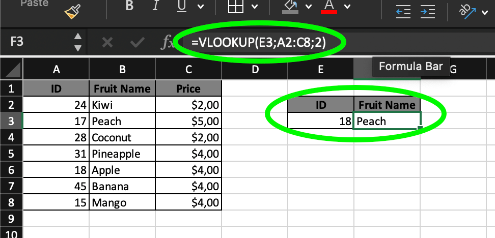
Solution

Enter FALSE as the last parameter if you are looking for an exact match. The correct VLOOKUP formula is

=VLOOKUP(E3,A2:C8,2,FALSE)

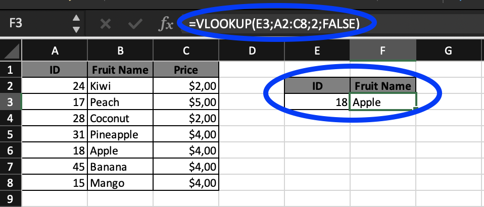
Explanation

The last parameter in the VLOOKUP function is Closest match (TRUE) or Exact match (FALSE). Most people are searching for a certain match such as for customer name, product name or employee name that need an exact match. FALSE should be entered for the last parameter in your VLOOKUP formula when you are looking for an exact value.

#2: The range in the VLOOKUP formula is not locked

Issue

When you drag your working Excel VLOOKUP formula down

=VLOOKUP(E3,A2:C8,2,FALSE)

it returns the #N/A error.

Solution

You need to lock the range in your VLOOKUP formula before dragging it or copying to other cells. To do this, type $ around the range as shown below: 

Your VLOOKUP formula should look like this:

=VLOOKUP(E3,$A$2:$C$8,2,FALSE)

Now you can drag it without any errors expected. 

Explanation

Once you dragged your VLOOKUP formula, the range in it changed, which caused the error.

#3: A new column has been inserted to the range

Issue

A new column was inserted and affected the range that was specified in your VLOOKUP formula. 

=VLOOKUP(E3,A2:C8,2,FALSE)

Solution

To avoid this in the future, you need to make the column number dynamic using the MATCH function. This allows you to retrieve the matched position of a lookup value and column number. In this way, any new inserted columns won’t affect your VLOOKUP formula.

We updated our formula, so it looks like this.

=VLOOKUP(F3,A2:D8,MATCH(G2,A1:D1,0),FALSE)

• G2 – the value to match in lookup range.
• A1:D1 – the lookup range.
• 0 – exact match type.

Let’s test the new lookup range by adding more columns as shown in the figure below:

The result does not change.

#4: Your table has gotten bigger

Issue

Your VLOOKUP formula was made for a specific limited range. You’ll have to update the formula manually every time when the range grows with new rows. Or not? 

Solution

Not only can you set the column dynamic, but also the range, by giving it a name. This will help you ensure your VLOOKUP function always checks the whole table by following these steps:

1. Select the range of cells you want to use for the lookup range. Click Home ? Format as Table and choose Orange, Table Style Medium 3 (or any other style you desire). 

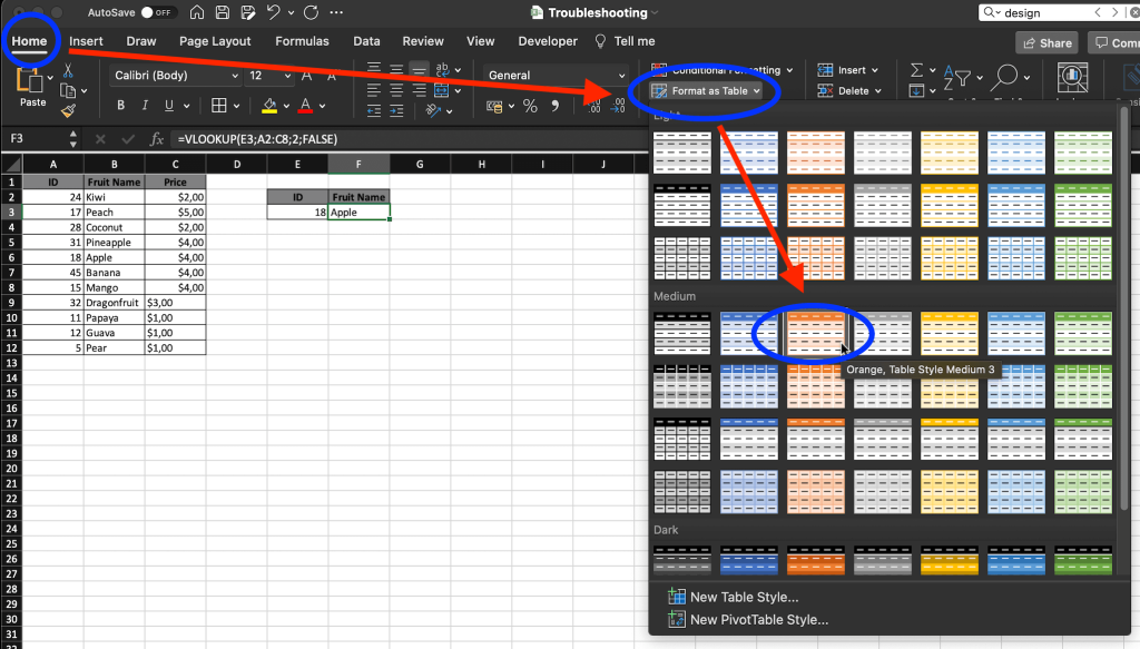
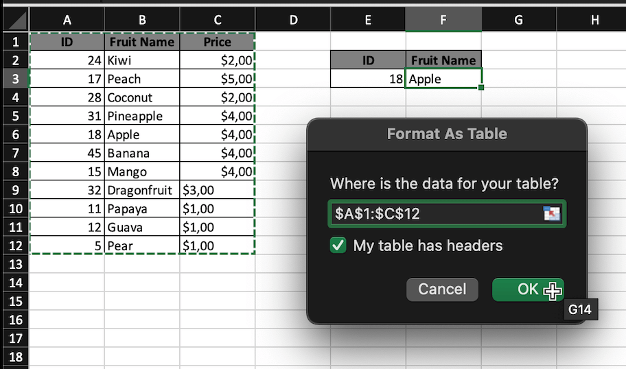
2. Specify your lookup range: $A$1:$C$12. Check the box My table has headers then click OK as shown in the screenshot below:

3. Update your lookup range in the VLOOKUP formula as follows:

Let’s test the new lookup range by adding one more row. Check your VLOOKUP by searching the new ID that you just added to the lookup range. The result returns the correct value as shown in figure below:

#5: Reverse VLOOKUP for those who do not have XLOOKUP in their version of Excel

Issue

The VLOOKUP formula cannot look up a value to the left, and your Excel does not have XLOOKUP.

Solution

You can vlookup to the left using the combination of the INDEX and MATCH functions:

1. Suppose you want to look up the ID for Coconut from the table below:

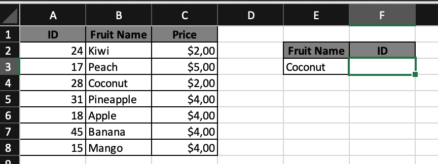
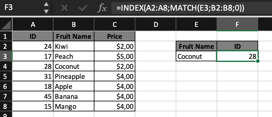
2. Type the following formula below in cell F3:

=INDEX(A2:A8,MATCH(E3,B2:B8,0))

• INDEX – a function in Excel that returns the value from a certain location in a range.
• A2:A8 – the range column where ID is stored is from A2-A8.
• MATCH – a function in Excel that used to locate the position of a lookup value in a table/column/row.
• E3 – where ‘Coconut’ is located.
• B2:B8 – the range column where Coconut is stored from B2:B8.
• 0 – an exact match of the return value.

3. The result is:

Is there any difference between VLOOKUP in Excel and Google Sheets

Basically, VLOOKUP in Excel and Google Sheets has the same logic and the same syntax. So, if you migrate to Excel from Google Sheets, you won’t have any troubles. But of course, there are some differences. Check out our blog posts about VLOOKUP in Google Sheets and Power BI VLOOKUP to find them. Good luck with looking up your data!